Differential equation: Difference between revisions
Implementing HTML-comment advice: general form before example for characteristic equations, complex-root demonstration, forced equations and variation of parameters shown with mathematics, step-by-step power-series and Laplace demonstrations. AI-assisted (RonzzWikiCowriter). (via update-page on MediaWiki MCP Server) |
No edit summary |
||
| (16 intermediate revisions by 2 users not shown) | |||
| Line 1: | Line 1: | ||
'''A differential equation''' is an equation that | '''A differential equation''' is an equation whose unknown is a function and which also involves that function's derivatives (rates of change). Where an ordinary equation such as $x^2=9$ is solved by numbers, a differential equation such as $y'+2y=0$ is solved by functions $y(x)$. | ||
A surprising number of laws of nature can be described by differential equations: pendulums, cooling drinks, growing populations, and discharging capacitors. | |||
== General and specific solution == | |||
The simplest differential equation prescribes the slope of a function $y(x)$: | |||
= | $$\frac{dy}{dx}=2x$$ | ||
Integrating both sides gives | |||
$$\int\frac{dy}{dx}\,dx=\int 2x\,dx\qquad\Longrightarrow\qquad y(x)=x^{2}+C$$ | |||
Where $C$ is an unknown constant. Therefore, the solution is not one single function, but a family of functions, known as the '''general solution'''. | |||
If we know the value of $y$ at a particular $x$, for instance, $y(0)=3$, then a '''particular solution''' function can be identified | |||
$$3=0^2+C\qquad\Longrightarrow\qquad C=3\qquad\Longrightarrow\qquad y=x^2+3$$ | |||
A prescribed value such as $y(a)=b$ allowing us to pin down a particular solution is called an '''initial condition'''. | |||
== Classifying differential equations == | |||
{{#content: | A differential equation can be classified by three criteria: its '''order''', its '''linearity''', and how many independent variables it involves. | ||
=== Order === | |||
The order is the order of the highest derivative present. | |||
$\frac{dy}{dx}=2x$ is first order, whereas Newton's second law, | |||
{{#content:Q1583}} | |||
is second order ($x(t)$ position of mass $m$, $F$ net force). | |||
=== Linearity and homogeneity === | |||
An equation is '''linear''' when the unknown and its derivatives appear only to the first power and never multiplied together. A linear first-order equation can always be written | |||
$$\frac{dy}{dx}+p(x)\,y=q(x)$$ | |||
= | It is said to be '''homogeneous''' when $q(x)=0$. | ||
<blockquote> | |||
The equations $dy/dx=y^2$ and $d^2\theta/dt^2+\sin\theta=0$ are nonlinear (square of $y$; sine of $\theta$). | |||
</blockquote> | |||
An important property of linear homogeneous equation is the '''superposition principle'''. If $y_1,y_2$ solve a homogeneous linear equation, so does $c_1y_1+c_2y_2$. | |||
== | For a nonlinear equation, the same principle usually does not apply: if $y'=y^2$ has two solutions $y_1'=y_1^2$ and $y_2'=y_2^2$ | ||
$$(y_1+y_2)'=y_1^2+y_2^2\neq (y_1+y_2)^2$$ | |||
so $y_1+y_2$ does not solve $y'=y^2$. | |||
=== Ordinary and partial === | |||
An '''ordinary differential equation''' (ODE) has one independent variable. A '''partial differential equation''' (PDE) has several, with partial derivatives. All the examples we have seen above are ordinary differential equations. For an example of a partial differential equation, we can take the heat equation describing the temperature $u$ of an insulated metal bar, according to position $x$ on the metal bar and time $t$ | |||
{{#content:Q1590}} | |||
where $\alpha$ is the thermal diffusivity. | |||
== | == Direction field == | ||
A first-order equation can be written | |||
{{#content:Q1581}} | |||
assigning to each point $(x,y)$ the slope $f(x,y)$ a solution must have there. Drawing short segments of that slope gives a '''direction field'''. Solution curves must run tangent to the direction field for every point they pass through. | |||
[[File:Slope field of exponential growth.png|thumb|Direction field of $dy/dx=y$. Credit: jjbeard (public domain).]] | |||
== Solving differential equations == | |||
Just like there is no general formula solving all algebraic equations, there is no general method permitting the solution of all differential equations. However, some standard methods exist for solving a restricted class of simple differential equations. | |||
=== First-order ODEs === | |||
==== Method 1: separable equations ==== | |||
'''General case.''' A first-order equation is separable when it can be rewritten as the equality of the derivative to the product of two functions, one containing only $x$, one containing only $y$. | |||
{{#content:Q1612}} | |||
after which both integrals can be evaluated directly. | |||
A quantity | '''Example: exponential growth and decay.''' A quantity whose rate of change is proportional to its own size, such as an unchecked population or a radioactive sample, obeys | ||
{{#content:Q1584}} | {{#content:Q1584}} | ||
Separating variables and integrating, | |||
{{ | $$\int\frac{dy}{y}=\int k\,dt\;\Longrightarrow\;\ln|y|=kt+C_1\;\Longrightarrow\;y=Ce^{kt}$$ | ||
The initial condition $y(0)=y_0$ fixes $C=y_0$, giving | |||
{{#content:Q1585}} (1) | |||
Newton's law of cooling | Observing (1) we notice this is very well an exponential growth (k>0)/decay(k<0). | ||
'''Example: Newton's law of cooling.''' A hot object in a cooler room loses heat through its surface, and the larger the temperature gap, the faster it cools: The temperature of the object is modelled by | |||
{{#content:Q1586}} | {{#content:Q1586}} | ||
Separating variables and integrating, | |||
$$\int\frac{dT}{T-T_a}=-k\int dt\;\Longrightarrow\;\ln|T-T_a|=-kt+C\;\Longrightarrow\;T-T_a=Ce^{-kt}$$ | |||
so with $T(0)=T_0$, hence $C=T_0-T_a$, | |||
$$T(t)=T_a+(T_0-T_a)e^{-kt}$$ | |||
==== Method 2: linear first-order equations (integrating factor) ==== | |||
'''General case.''' For the linear equation | |||
$$y'+p(x)\,y=q(x)$$ | |||
introduce the integrating factor $\mu=e^{\int p\,dx}$, chosen so that $\mu'=p\mu$; multiplying by $\mu$ collapses the left-hand side into a single derivative: | |||
{{#content:Q1613}} | |||
Integrating both sides, | |||
$$\mu y=\int\mu\,q\,dx+C\;\Longrightarrow\;y=\frac{1}{\mu}\int\mu\,q\,dx+\frac{C}{\mu}$$ | |||
If you notice, the first term $y=\frac{1}{\mu}\int\mu\,q\,dx$$\frac{C}{\mu}$ provides one particular solution to the non-homogeneous equation, and the second term, $C/\mu=Ce^{-\int p\,dx}$, is a solution to the homogeneous counter par of the original equation: $y'+p(x)\,y=0$. It generalises the solution to the entire solution family. | |||
This is in fact a general principle: $y=y_p+y_h$, i.e., the solution family of a non-homogeneous equation is the sum of one particular solution plus the solution to its homogeneous counterpart. | |||
To see the method in action, consider | |||
$$ \frac{dy}{dx} + \frac{1}{x}\,y = x^2, \qquad x>0. $$ | |||
Here $P(x)=1/x$, so | |||
== | $$ \mu(x)=e^{\int \frac{1}{x}\,dx}=e^{\ln x}=x. $$ | ||
= | Multiply the whole equation by $\mu(x)=x$: | ||
$$ x\frac{dy}{dx} + y = x^3. $$ | |||
The left side is exactly the derivative of the product $x\,y$: | |||
$$ \frac{d}{dx}\bigl(xy\bigr) = x^3. $$ | |||
Integrate with respect to $x$: | |||
$$ xy = \int x^3\,dx = \frac{x^4}{4} + C. $$ | |||
Finally, divide by $x$ to obtain the general solution: | |||
= | $$ y = \frac{x^3}{4} + \frac{C}{x}. $$ | ||
A quick substitution verifies that this function family satisfies the original equation. The arbitrary constant $C$ can be determined later if an initial condition $y(x_0)=y_0$ is given. | |||
==== Method 3: constant-coefficient linear equations (trial solutions) ==== | |||
=== Second-order ODEs === | |||
==== Method 1: direct integration ==== | |||
= | '''General case.''' For $y''=f(x)$, | ||
$$y''=f(x)\;\Longrightarrow\;y'=\int f(x)\,dx+C_1\;\Longrightarrow\;y=\int\!\!\left(\int f(x)\,dx\right)dx+C_1x+C_2$$ | |||
= | and likewise $y^{(n)}=f(x)$ by $n$ integrations. | ||
''' | '''Example: free fall.''' A ball released above the ground falls under gravity alone, which accelerates it downward at the constant rate $g\approx 9.8\ \mathrm{m\,s^{-2}}$; Newton's second law gives the second-order equation $x''=-g$, of the form above with $f(x)=-g$. Integrating twice, | ||
{{ | $$x''=-9.8\;\Longrightarrow\;\frac{dx}{dt}=-9.8t+v_0\;\Longrightarrow\;x(t)=-4.9t^2+v_0t+x_0$$ | ||
Numeric scenario: the ball is dropped from rest, $v_0=0$, at height $x_0=19.6\ \mathrm{m}$. It reaches the ground, $x=0$, when | |||
{{ | $$0=19.6-4.9t^2\;\Longrightarrow\;t=\sqrt{19.6/4.9}=2\ \text{s}$$ | ||
so the two initial conditions have pinned down the whole trajectory. | |||
==== Method 2: linear equations with constant coefficients ==== | |||
'''General case.''' | |||
$$y''+a\,y'+b\,y=f(x)$$ | |||
''' | '''Homogeneous case ($f=0$).''' The exponential trial $y=e^{rx}$, | ||
{{#content:Q1644}} | {{#content:Q1644}} | ||
gives the characteristic equation $r^2+ar+b=0$, whose roots determine $y_h$: | |||
{{ | * $r_1\neq r_2$ real: $y_h=C_1e^{r_1x}+C_2e^{r_2x}$; | ||
* $r_1=r_2=r$: $y_h=(C_1+C_2x)e^{rx}$; | |||
* $r=\alpha\pm i\beta$: $y_h=e^{\alpha x}(C_1\cos\beta x+C_2\sin\beta x)$. | |||
'''Non-homogeneous case ($f\neq 0$).''' $y=y_h+y_p$, with $y_p$ found by undetermined coefficients as in Method 3. | |||
'''Worked demonstration (homogeneous).''' $y''-3y'+2y=0$: $r^2-3r+2=(r-1)(r-2)=0$, | |||
{{#content:Q1608}} | {{#content:Q1608}} | ||
Check: $e^x$ gives $(1-3+2)e^x=0$. | |||
{{ | '''Worked demonstration (non-homogeneous).''' $y''-3y'+2y=2e^{3x}$: keep $y_h$ above, try $y_p=Ae^{3x}$: | ||
$$y_p''-3y_p'+2y_p=(9-9+2)Ae^{3x}=2Ae^{3x}\;\Longrightarrow\;A=1$$ | |||
{{ | $$y=C_1e^x+C_2e^{2x}+e^{3x}$$ | ||
'''Example: the harmonic oscillator (a mass on a spring).''' A mass attached to a spring is pulled back towards its rest position by a force $-kx$ proportional to the displacement (Hooke's law); once released it oscillates. Newton's second law models the motion, | |||
{{ | $$m\frac{d^2x}{dt^2}=-kx\;\Longrightarrow\;x''+\omega_0^2x=0,\qquad \omega_0=\sqrt{\frac{k}{m}}$$ | ||
{{#content:Q1588}} | |||
The trial $x=e^{rt}$ gives the characteristic equation $r^2+\omega_0^2=0$ with roots $r=\pm i\omega_0$, the complex-pair case with $\alpha=0$, hence | |||
$$x(t)=A\cos\omega_0t+B\sin\omega_0t$$ | |||
with $A,B$ fixed by the initial position and velocity. | |||
[[File:Simple harmonic motion animation.gif|thumb|A mass on a spring: the harmonic oscillator solution is a sinusoid of fixed amplitude. Credit: Evil saltine (public domain).]] | |||
Numeric scenario: a mass $m=2\ \mathrm{kg}$ hangs on a spring with $k=8\ \mathrm{N\,m^{-1}}$, so $\omega_0=\sqrt{8/2}=2\ \mathrm{rad\,s^{-1}}$ and the displacement obeys $x''+4x=0$. Pulled $0.10\ \mathrm{m}$ from rest and released, the conditions $x(0)=0.10$, $x'(0)=0$ give $A=0.10$, $B=0$: | |||
{{ | $$x(t)=0.10\cos 2t\ \mathrm{m},\qquad P=\frac{2\pi}{\omega_0}=\pi\approx 3.14\ \text{s}$$ | ||
After one second $x(1)=0.10\cos 2\approx -0.042\ \mathrm{m}$, and the motion is '''simple harmonic motion'''.<ref>{{#cite:Q1577}}</ref> | |||
=== Partial differential equations === | |||
Two standard techniques give closed-form solutions of linear PDEs: separation of variables, for separable problems on bounded domains, and the method of characteristics, for first-order equations. The wave equation is also solved by the second technique, because its operator factors into two first-order parts. Both methods below are stated in general and then applied to a concrete equation. | |||
==== Method 1: separation of variables ==== | |||
'''General form.''' For a linear homogeneous PDE in two variables on a bounded domain with homogeneous boundary conditions, seek a solution of the separated form | |||
$$u(x,t)=X(x)\,T(t)$$ | |||
Substituting into the PDE and dividing by $XT$ separates the variables into one ordinary differential equation in $x$ and one in $t$. Since the two sides are functions of different variables, they can be identically equal only if each equals the same constant, the separation constant $-\lambda$. The $x$-equation together with the boundary conditions is an eigenvalue problem: only a discrete sequence of constants $\lambda_n$, with eigenfunctions $X_n(x)$, is admissible. The $t$-equation then has a solution $T_n(t)$ for each $n$, and every product $X_nT_n$ solves the PDE. | |||
'''General algebraic solution.''' The PDE is linear and homogeneous, so the separated modes superimpose: | |||
$$u(x,t)=\sum_n c_n\,X_n(x)\,T_n(t)$$ | |||
with the coefficients $c_n$ chosen so that the series equals the initial profile $u(x,0)$; orthogonality of the eigenfunctions $X_n$ determines them. | |||
'''Example: the heat equation.''' The temperature of a bar of length $L$ with insulated sides and both ends held at $0$ obeys | |||
{{ | $$\frac{\partial u}{\partial t}=\alpha\frac{\partial^2u}{\partial x^2},\qquad u(0,t)=u(L,t)=0$$ | ||
Substituting $u=X(x)T(t)$ gives $XT'=\alpha X''T$, and dividing by $\alpha XT$, | |||
{{#content: | {{#content:Q1622}} | ||
The $t$-equation $T'=-\alpha\lambda T$ has solution $T=e^{-\alpha\lambda t}$, and the $x$-equation | |||
$$X''=-\lambda X\;\Longrightarrow\;X=A\cos(\sqrt\lambda\,x)+B\sin(\sqrt\lambda\,x)$$ | |||
together with the boundary conditions forces $X(0)=X(L)=0$: hence $A=0$ and $\sin(\sqrt\lambda\,L)=0$, so $\sqrt\lambda\,L=n\pi$, $n=1,2,\dots$. Each $\lambda=(n\pi/L)^2$ gives one mode | |||
{{ | $$u_n(x,t)=\sin\frac{n\pi x}{L}\,e^{-\alpha(n\pi/L)^2t}$$ | ||
and the general algebraic solution above becomes | |||
{{#content:Q1611}} | {{#content:Q1611}} | ||
with $b_n$ determined by the Fourier sine series of the initial profile $u(x,0)$; the decay rate $\alpha(n\pi/L)^2$ grows as $n^2$. | |||
Numeric scenario: a $1\ \mathrm{m}$ iron bar, heated so that its centre is at $100\,^{\circ}\mathrm{C}$ while both ends are held at $0\,^{\circ}\mathrm{C}$, cools by conduction with iron's diffusivity $\alpha\approx 2.3\times10^{-5}\ \mathrm{m^2s^{-1}}$. The initial profile $u(x,0)=100\sin(\pi x/L)$ is exactly the first mode, so only $n=1$ contributes and | |||
$$u(x,t)=100\sin\frac{\pi x}{L}\,e^{-\alpha\pi^2t/L^2}$$ | |||
At the centre, with $L=1$ and $\alpha\pi^2\approx 2.3\times10^{-4}\ \text{s}^{-1}$, | |||
$$u\!\left(\tfrac12,t\right)=100\,e^{-2.3\times10^{-4}t}$$ | |||
so after one hour $u\approx 100e^{-0.82}\approx 44\,^{\circ}\mathrm{C}$, and $50\,^{\circ}\mathrm{C}$ is reached at $t=\ln 2/(2.3\times10^{-4})\approx 3050\ \text{s}\approx 51$ min.<ref>{{#cite:Q1579}}</ref> | |||
==== Method 2: the method of characteristics ==== | |||
'''General form.''' The method of characteristics solves first-order PDEs by tracing curves along which the PDE reduces to ordinary differential equations. In two independent variables the general quasilinear first-order equation is | |||
$$A(x,t,u)\,u_x+B(x,t,u)\,u_t=C(x,t,u)$$ | |||
A solution $u=u(x,t)$ is a surface in $(x,t,u)$-space. Its tangent plane at each point is spanned by $(1,0,u_x)$ and $(0,1,u_t)$, so a vector $(A,B,C)$ is tangent to the surface exactly when $C=A u_x+B u_t$, the condition expressed by the PDE itself. The solution surface is therefore swept out by the integral curves of the vector field $(A,B,C)$, the characteristic curves, which solve the characteristic system of ordinary differential equations | |||
$$\frac{dx}{ds}=A(x,t,u),\qquad \frac{dt}{ds}=B(x,t,u),\qquad \frac{du}{ds}=C(x,t,u)$$ | |||
Given data on a curve that is not itself characteristic, such as $u(x,0)=u_0(x)$, one characteristic issues from each point of the curve, and integrating the system carries the data across the region the characteristics cover. For the linear homogeneous case | |||
$$a(x,t)\,u_x+b(x,t)\,u_t=0$$ | |||
the $x$- and $t$-equations do not involve $u$, and the third gives $du/ds=0$: the solution is constant along each characteristic. The characteristics form a one-parameter family; let $\psi(x,t)=\text{const}$ be a first integral, a function constant on each member of the family. | |||
'''General algebraic solution.''' Since $u$ is constant on every characteristic and the characteristics are the level sets of $\psi$, the general solution is an arbitrary function of the first integral, | |||
= | $$u(x,t)=F\bigl(\psi(x,t)\bigr)$$ | ||
When | with $F$ fixed by the initial data. When the right-hand side of the PDE is nonzero, $u$ changes along a characteristic at the rate $C$ (or of the given source term), so the general solution acquires an integral of that term along the curve. | ||
{ | '''Example: transport of a pollutant.''' For constant coefficients $c$ the equation $u_t+c\,u_x=0$ has characteristics $dx/dt=c$, the straight lines $x-ct=\text{const}$; hence $\psi=x-ct$, and the general algebraic solution is the travelling wave | ||
$$u(x,t)=F(x-ct),\qquad u(x,0)=F(x)$$ | |||
{{ | A river flows steadily at speed $c=2\ \mathrm{m\,s^{-1}}$, and a factory releases a concentrated slug of pollutant at one point; as long as mixing and diffusion are negligible, the current simply carries the whole slug downstream without changing it. The concentration obeys $u_t+2u_x=0$ with the Gaussian initial profile | ||
$$u(x,0)=50\,e^{-(x/10)^2}\ \mathrm{mg\,L^{-1}}$$ | |||
(peak $50\ \mathrm{mg\,L^{-1}}$ at the release point, falling by $e^{-1}$ ten metres away). The solution above gives | |||
{{ | $$u(x,t)=50\,e^{-((x-2t)/10)^2}\ \mathrm{mg\,L^{-1}}$$ | ||
After one minute the peak has moved from $x=0$ to $x=ct=120\ \mathrm{m}$, still reading $50\ \mathrm{mg\,L^{-1}}$; pure transport does not spread the slug, which would require the second-order term $\alpha u_{xx}$ of the heat equation. With a source $q(x,t)$, the value accumulates along each characteristic: | |||
= | $$u(x,t)=F(x-ct)+\int_0^t q\bigl(x-c(t-\tau),\tau\bigr)\,d\tau$$ | ||
'''Example: the wave equation.''' The wave equation | |||
$$u_{tt}=c^2u_{xx}$$ | |||
is second order, yet its operator factors into two first-order transport operators, so the method of characteristics still applies. Introduce the characteristic coordinates | |||
$$\xi=x-ct,\qquad \eta=x+ct$$ | |||
{{ | in which the operator becomes $u_{tt}-c^2u_{xx}=-4c^2u_{\xi\eta}$, so the equation reads $u_{\xi\eta}=0$. Hence $u_\xi$ depends on $\xi$ alone, and one further integration gives the general algebraic solution (d'Alembert, 1747): | ||
$$u(x,t)=f(x-ct)+g(x+ct)$$ | |||
a superposition of two travelling waves, one in each direction. The functions $f,g$ are fixed by the initial displacement and velocity: for a string released from rest with initial displacement $\phi(x)$, the conditions $u(x,0)=\phi(x)$ and $u_t(x,0)=0$ give $f=g=\phi/2$, so | |||
$$u(x,t)=\frac{\phi(x-ct)+\phi(x+ct)}{2}$$ | |||
and the initial hump separates into two half-size copies travelling apart at speed $c$.<ref>{{#cite:Q1579}}</ref> | |||
=== When no formula exists === | |||
Most equations, especially nonlinear ones, fit none of the classes above and have no solution in terms of familiar functions. They are studied in one of three ways:<ref>{{#cite:Q1576}}</ref><ref>{{#cite:Q1578}}</ref> | |||
* '''Numerically''', when numbers suffice: [[Euler's method]] steps along the slope field; | |||
* '''[[Qualitative methods]]''': equilibria, stability and long-term behaviour, without formulas; | |||
* '''Series and transforms''', for linear cases: [[Power series]] or the [[Laplace transform]]. | |||
{{ | <uml type="uml"> | ||
@startuml | |||
skinparam monochrome true | |||
start | |||
:You have a differential equation; | |||
if (First order and separable?\ny' = g(x) h(y)?) then (yes) | |||
:Separate and integrate:\n∫ dy/h(y) = ∫ g(x) dx; | |||
else (no) | |||
if (First order and linear?\ny' + p(x) y = q(x)?) then (yes) | |||
if (Constant coefficients?\ny' + a y = q(x)?) then (yes) | |||
:Trial solution:\ny_h = C e^{-ax} + guessed y_p; | |||
else (no) | |||
:Integrating factor\nμ = e^{∫ p dx}; | |||
endif | |||
else (no) | |||
if (Second order, of the form\ny'' = f(x)?) then (yes) | |||
:Integrate twice; | |||
else (no) | |||
if (Second order, linear, constant coefficients?\ny'' + a y' + b y = 0? or = f(x)?) then (yes) | |||
:Characteristic equation\nr² + a r + b = 0;\nthen add a particular y_p; | |||
else (no) | |||
if (Transport equation?\nu_t + c u_x = 0?) then (yes) | |||
:Travelling wave\nu(x,t) = f(x - ct); | |||
else (no) | |||
if (Linear PDE on a simple shape,\ne.g. the heat equation?) then (yes) | |||
:Separate variables\nu(x,t) = X(x) T(t); | |||
else (no) | |||
if (Are approximate numbers enough?) then (yes) | |||
:Numerical stepping\n(Euler's method); | |||
else (no) | |||
if (Linear?) then (yes) | |||
:Power series or Laplace transform; | |||
else (no) | |||
:Qualitative study:\nequilibria, stability, chaos; | |||
endif | |||
endif | |||
endif | |||
endif | |||
endif | |||
endif | |||
endif | |||
endif | |||
stop | |||
@enduml | |||
</uml> | |||
The exact methods occupy the branches on the left; most equations encountered in research fall through to the routes on the right, each treated in its own article. | |||
== | == A short history == | ||
The origins of differential equations coincide with those of the calculus, since the calculus supplies the language in which rates of change are expressed and inverted. Newton's laws of motion and of universal gravitation, published in the ''Philosophiae Naturalis Principia Mathematica'' (1687), are differential equations; Newton treated them by the geometrical and infinite-series methods of his fluxional calculus. Although Newton developed a notation for fluxions, the differential notation $dy/dx$ introduced by Leibniz in the 1670s proved the more enduring: it exhibits the structure of the equation directly and is the notation adopted in this article.<ref>{{#cite:Q1577}}</ref> | |||
[[File:Isaac Newton portrait.jpg|thumb|left|Isaac Newton (portrait after Godfrey Kneller, 1689). Newton's laws of motion and of gravitation (''Principia'', 1687) are differential equations. Credit: James Thronill after Godfrey Kneller (public domain).]] | |||
The consolidation of these techniques into a systematic theory is due in large measure to [[Person:Leonhard Euler|Leonhard Euler]], whose work in the middle decades of the eighteenth century established the principal exact methods. Euler showed that linear equations with constant coefficients are solved by the substitution $y=e^{rx}$, which reduces the problem to an algebraic equation, and he advanced the theory of series solutions. For equations that admitted no closed-form solution, he introduced the step-by-step numerical procedure, described above as Euler's method, that bears his name. The exact methods presented in this article derive, in large part, from his work.<ref>{{#cite:Q1577}}</ref> | |||
[[File:Leonhard Euler portrait.jpg|thumb|Leonhard Euler (portrait by Jakob Emanuel Handmann, 1753) | [[File:Leonhard Euler portrait.jpg|thumb|Leonhard Euler (portrait by Jakob Emanuel Handmann, 1753). Credit: Jakob Emanuel Handmann (public domain).]] | ||
The theory of partial differential equations arose from the demands of eighteenth-century physics. In 1747, [[Person:Jean le Rond d'Alembert|Jean le Rond d'Alembert]] derived the wave equation for the vibrating string and established that its general solution consists of two waves propagating in opposite directions. The problem of heat conduction proved more demanding, because the initial temperature distribution of a conducting body is arbitrary. In his ''Théorie analytique de la chaleur'' (1822), [[Person:Joseph Fourier|Joseph Fourier]] derived the heat equation from the physical principles of conduction and solved it by expanding the initial data into a trigonometric series. This work established separation of variables as a standard technique of mathematical physics, and the Fourier series introduced for the purpose has since become fundamental to the analysis of periodic phenomena, from acoustics to signal processing.<ref>{{#cite:Q1579}}</ref> | |||
The | The limits of closed-form methods became apparent towards the end of the nineteenth century, and the later history of the subject is concerned principally with equations for which elementary solutions do not exist. In his investigation of the three-body problem of celestial mechanics, [[Person:Henri Poincaré|Henri Poincaré]] demonstrated that qualitative properties of the motion, such as its equilibria, stability, and long-term behaviour, can be characterised without solving the equations, thereby founding the qualitative theory of dynamical systems. The subsequent development of electronic computing made numerical approximation, of which Euler's method is the simplest instance, a routine and general technique. The two strands converged in 1963, when [[Person:Edward Lorenz|Edward Lorenz]], studying a simplified system of three ordinary differential equations that models atmospheric convection, established the phenomenon of deterministic chaos: although the equations are deterministic, their solutions are aperiodic and depend so sensitively on initial conditions that long-term weather prediction is not feasible in practice. These later approaches, qualitative analysis, numerical approximation, and series and transform methods, are treated in dedicated articles.<ref>{{#cite:Q1578}}</ref> | ||
== References == | == References == | ||
Latest revision as of 11:56, 7 September 2026
A differential equation is an equation whose unknown is a function and which also involves that function's derivatives (rates of change). Where an ordinary equation such as $x^2=9$ is solved by numbers, a differential equation such as $y'+2y=0$ is solved by functions $y(x)$.
A surprising number of laws of nature can be described by differential equations: pendulums, cooling drinks, growing populations, and discharging capacitors.
General and specific solution
The simplest differential equation prescribes the slope of a function $y(x)$:
$$\frac{dy}{dx}=2x$$
Integrating both sides gives
$$\int\frac{dy}{dx}\,dx=\int 2x\,dx\qquad\Longrightarrow\qquad y(x)=x^{2}+C$$
Where $C$ is an unknown constant. Therefore, the solution is not one single function, but a family of functions, known as the general solution.
If we know the value of $y$ at a particular $x$, for instance, $y(0)=3$, then a particular solution function can be identified
$$3=0^2+C\qquad\Longrightarrow\qquad C=3\qquad\Longrightarrow\qquad y=x^2+3$$
A prescribed value such as $y(a)=b$ allowing us to pin down a particular solution is called an initial condition.
Classifying differential equations
A differential equation can be classified by three criteria: its order, its linearity, and how many independent variables it involves.
Order
The order is the order of the highest derivative present.
$\frac{dy}{dx}=2x$ is first order, whereas Newton's second law,
is second order ($x(t)$ position of mass $m$, $F$ net force).
Linearity and homogeneity
An equation is linear when the unknown and its derivatives appear only to the first power and never multiplied together. A linear first-order equation can always be written
$$\frac{dy}{dx}+p(x)\,y=q(x)$$
It is said to be homogeneous when $q(x)=0$.
The equations $dy/dx=y^2$ and $d^2\theta/dt^2+\sin\theta=0$ are nonlinear (square of $y$; sine of $\theta$).
An important property of linear homogeneous equation is the superposition principle. If $y_1,y_2$ solve a homogeneous linear equation, so does $c_1y_1+c_2y_2$.
For a nonlinear equation, the same principle usually does not apply: if $y'=y^2$ has two solutions $y_1'=y_1^2$ and $y_2'=y_2^2$
$$(y_1+y_2)'=y_1^2+y_2^2\neq (y_1+y_2)^2$$
so $y_1+y_2$ does not solve $y'=y^2$.
Ordinary and partial
An ordinary differential equation (ODE) has one independent variable. A partial differential equation (PDE) has several, with partial derivatives. All the examples we have seen above are ordinary differential equations. For an example of a partial differential equation, we can take the heat equation describing the temperature $u$ of an insulated metal bar, according to position $x$ on the metal bar and time $t$
where $\alpha$ is the thermal diffusivity.
Direction field
A first-order equation can be written
assigning to each point $(x,y)$ the slope $f(x,y)$ a solution must have there. Drawing short segments of that slope gives a direction field. Solution curves must run tangent to the direction field for every point they pass through.

Solving differential equations
Just like there is no general formula solving all algebraic equations, there is no general method permitting the solution of all differential equations. However, some standard methods exist for solving a restricted class of simple differential equations.
First-order ODEs
Method 1: separable equations
General case. A first-order equation is separable when it can be rewritten as the equality of the derivative to the product of two functions, one containing only $x$, one containing only $y$.
after which both integrals can be evaluated directly.
Example: exponential growth and decay. A quantity whose rate of change is proportional to its own size, such as an unchecked population or a radioactive sample, obeys
Separating variables and integrating,
$$\int\frac{dy}{y}=\int k\,dt\;\Longrightarrow\;\ln|y|=kt+C_1\;\Longrightarrow\;y=Ce^{kt}$$
The initial condition $y(0)=y_0$ fixes $C=y_0$, giving
(1)
Observing (1) we notice this is very well an exponential growth (k>0)/decay(k<0).
Example: Newton's law of cooling. A hot object in a cooler room loses heat through its surface, and the larger the temperature gap, the faster it cools: The temperature of the object is modelled by
Separating variables and integrating,
$$\int\frac{dT}{T-T_a}=-k\int dt\;\Longrightarrow\;\ln|T-T_a|=-kt+C\;\Longrightarrow\;T-T_a=Ce^{-kt}$$
so with $T(0)=T_0$, hence $C=T_0-T_a$,
$$T(t)=T_a+(T_0-T_a)e^{-kt}$$
Method 2: linear first-order equations (integrating factor)
General case. For the linear equation
$$y'+p(x)\,y=q(x)$$
introduce the integrating factor $\mu=e^{\int p\,dx}$, chosen so that $\mu'=p\mu$; multiplying by $\mu$ collapses the left-hand side into a single derivative:
Integrating both sides,
$$\mu y=\int\mu\,q\,dx+C\;\Longrightarrow\;y=\frac{1}{\mu}\int\mu\,q\,dx+\frac{C}{\mu}$$
If you notice, the first term $y=\frac{1}{\mu}\int\mu\,q\,dx$$\frac{C}{\mu}$ provides one particular solution to the non-homogeneous equation, and the second term, $C/\mu=Ce^{-\int p\,dx}$, is a solution to the homogeneous counter par of the original equation: $y'+p(x)\,y=0$. It generalises the solution to the entire solution family.
This is in fact a general principle: $y=y_p+y_h$, i.e., the solution family of a non-homogeneous equation is the sum of one particular solution plus the solution to its homogeneous counterpart.
To see the method in action, consider
$$ \frac{dy}{dx} + \frac{1}{x}\,y = x^2, \qquad x>0. $$
Here $P(x)=1/x$, so
$$ \mu(x)=e^{\int \frac{1}{x}\,dx}=e^{\ln x}=x. $$
Multiply the whole equation by $\mu(x)=x$:
$$ x\frac{dy}{dx} + y = x^3. $$
The left side is exactly the derivative of the product $x\,y$:
$$ \frac{d}{dx}\bigl(xy\bigr) = x^3. $$
Integrate with respect to $x$:
$$ xy = \int x^3\,dx = \frac{x^4}{4} + C. $$
Finally, divide by $x$ to obtain the general solution:
$$ y = \frac{x^3}{4} + \frac{C}{x}. $$
A quick substitution verifies that this function family satisfies the original equation. The arbitrary constant $C$ can be determined later if an initial condition $y(x_0)=y_0$ is given.
Method 3: constant-coefficient linear equations (trial solutions)
Second-order ODEs
Method 1: direct integration
General case. For $y''=f(x)$,
$$y''=f(x)\;\Longrightarrow\;y'=\int f(x)\,dx+C_1\;\Longrightarrow\;y=\int\!\!\left(\int f(x)\,dx\right)dx+C_1x+C_2$$
and likewise $y^{(n)}=f(x)$ by $n$ integrations.
Example: free fall. A ball released above the ground falls under gravity alone, which accelerates it downward at the constant rate $g\approx 9.8\ \mathrm{m\,s^{-2}}$; Newton's second law gives the second-order equation $x''=-g$, of the form above with $f(x)=-g$. Integrating twice,
$$x''=-9.8\;\Longrightarrow\;\frac{dx}{dt}=-9.8t+v_0\;\Longrightarrow\;x(t)=-4.9t^2+v_0t+x_0$$
Numeric scenario: the ball is dropped from rest, $v_0=0$, at height $x_0=19.6\ \mathrm{m}$. It reaches the ground, $x=0$, when
$$0=19.6-4.9t^2\;\Longrightarrow\;t=\sqrt{19.6/4.9}=2\ \text{s}$$
so the two initial conditions have pinned down the whole trajectory.
Method 2: linear equations with constant coefficients
General case.
$$y''+a\,y'+b\,y=f(x)$$
Homogeneous case ($f=0$). The exponential trial $y=e^{rx}$,
gives the characteristic equation $r^2+ar+b=0$, whose roots determine $y_h$:
- $r_1\neq r_2$ real: $y_h=C_1e^{r_1x}+C_2e^{r_2x}$;
- $r_1=r_2=r$: $y_h=(C_1+C_2x)e^{rx}$;
- $r=\alpha\pm i\beta$: $y_h=e^{\alpha x}(C_1\cos\beta x+C_2\sin\beta x)$.
Non-homogeneous case ($f\neq 0$). $y=y_h+y_p$, with $y_p$ found by undetermined coefficients as in Method 3.
Worked demonstration (homogeneous). $y''-3y'+2y=0$: $r^2-3r+2=(r-1)(r-2)=0$,
Check: $e^x$ gives $(1-3+2)e^x=0$.
Worked demonstration (non-homogeneous). $y''-3y'+2y=2e^{3x}$: keep $y_h$ above, try $y_p=Ae^{3x}$:
$$y_p''-3y_p'+2y_p=(9-9+2)Ae^{3x}=2Ae^{3x}\;\Longrightarrow\;A=1$$
$$y=C_1e^x+C_2e^{2x}+e^{3x}$$
Example: the harmonic oscillator (a mass on a spring). A mass attached to a spring is pulled back towards its rest position by a force $-kx$ proportional to the displacement (Hooke's law); once released it oscillates. Newton's second law models the motion,
$$m\frac{d^2x}{dt^2}=-kx\;\Longrightarrow\;x''+\omega_0^2x=0,\qquad \omega_0=\sqrt{\frac{k}{m}}$$
The trial $x=e^{rt}$ gives the characteristic equation $r^2+\omega_0^2=0$ with roots $r=\pm i\omega_0$, the complex-pair case with $\alpha=0$, hence
$$x(t)=A\cos\omega_0t+B\sin\omega_0t$$
with $A,B$ fixed by the initial position and velocity.

Numeric scenario: a mass $m=2\ \mathrm{kg}$ hangs on a spring with $k=8\ \mathrm{N\,m^{-1}}$, so $\omega_0=\sqrt{8/2}=2\ \mathrm{rad\,s^{-1}}$ and the displacement obeys $x''+4x=0$. Pulled $0.10\ \mathrm{m}$ from rest and released, the conditions $x(0)=0.10$, $x'(0)=0$ give $A=0.10$, $B=0$:
$$x(t)=0.10\cos 2t\ \mathrm{m},\qquad P=\frac{2\pi}{\omega_0}=\pi\approx 3.14\ \text{s}$$
After one second $x(1)=0.10\cos 2\approx -0.042\ \mathrm{m}$, and the motion is simple harmonic motion.[1]
Partial differential equations
Two standard techniques give closed-form solutions of linear PDEs: separation of variables, for separable problems on bounded domains, and the method of characteristics, for first-order equations. The wave equation is also solved by the second technique, because its operator factors into two first-order parts. Both methods below are stated in general and then applied to a concrete equation.
Method 1: separation of variables
General form. For a linear homogeneous PDE in two variables on a bounded domain with homogeneous boundary conditions, seek a solution of the separated form
$$u(x,t)=X(x)\,T(t)$$
Substituting into the PDE and dividing by $XT$ separates the variables into one ordinary differential equation in $x$ and one in $t$. Since the two sides are functions of different variables, they can be identically equal only if each equals the same constant, the separation constant $-\lambda$. The $x$-equation together with the boundary conditions is an eigenvalue problem: only a discrete sequence of constants $\lambda_n$, with eigenfunctions $X_n(x)$, is admissible. The $t$-equation then has a solution $T_n(t)$ for each $n$, and every product $X_nT_n$ solves the PDE.
General algebraic solution. The PDE is linear and homogeneous, so the separated modes superimpose:
$$u(x,t)=\sum_n c_n\,X_n(x)\,T_n(t)$$
with the coefficients $c_n$ chosen so that the series equals the initial profile $u(x,0)$; orthogonality of the eigenfunctions $X_n$ determines them.
Example: the heat equation. The temperature of a bar of length $L$ with insulated sides and both ends held at $0$ obeys
$$\frac{\partial u}{\partial t}=\alpha\frac{\partial^2u}{\partial x^2},\qquad u(0,t)=u(L,t)=0$$
Substituting $u=X(x)T(t)$ gives $XT'=\alpha X''T$, and dividing by $\alpha XT$,
The $t$-equation $T'=-\alpha\lambda T$ has solution $T=e^{-\alpha\lambda t}$, and the $x$-equation
$$X''=-\lambda X\;\Longrightarrow\;X=A\cos(\sqrt\lambda\,x)+B\sin(\sqrt\lambda\,x)$$
together with the boundary conditions forces $X(0)=X(L)=0$: hence $A=0$ and $\sin(\sqrt\lambda\,L)=0$, so $\sqrt\lambda\,L=n\pi$, $n=1,2,\dots$. Each $\lambda=(n\pi/L)^2$ gives one mode
$$u_n(x,t)=\sin\frac{n\pi x}{L}\,e^{-\alpha(n\pi/L)^2t}$$
and the general algebraic solution above becomes
with $b_n$ determined by the Fourier sine series of the initial profile $u(x,0)$; the decay rate $\alpha(n\pi/L)^2$ grows as $n^2$.
Numeric scenario: a $1\ \mathrm{m}$ iron bar, heated so that its centre is at $100\,^{\circ}\mathrm{C}$ while both ends are held at $0\,^{\circ}\mathrm{C}$, cools by conduction with iron's diffusivity $\alpha\approx 2.3\times10^{-5}\ \mathrm{m^2s^{-1}}$. The initial profile $u(x,0)=100\sin(\pi x/L)$ is exactly the first mode, so only $n=1$ contributes and
$$u(x,t)=100\sin\frac{\pi x}{L}\,e^{-\alpha\pi^2t/L^2}$$
At the centre, with $L=1$ and $\alpha\pi^2\approx 2.3\times10^{-4}\ \text{s}^{-1}$,
$$u\!\left(\tfrac12,t\right)=100\,e^{-2.3\times10^{-4}t}$$
so after one hour $u\approx 100e^{-0.82}\approx 44\,^{\circ}\mathrm{C}$, and $50\,^{\circ}\mathrm{C}$ is reached at $t=\ln 2/(2.3\times10^{-4})\approx 3050\ \text{s}\approx 51$ min.[2]
Method 2: the method of characteristics
General form. The method of characteristics solves first-order PDEs by tracing curves along which the PDE reduces to ordinary differential equations. In two independent variables the general quasilinear first-order equation is
$$A(x,t,u)\,u_x+B(x,t,u)\,u_t=C(x,t,u)$$
A solution $u=u(x,t)$ is a surface in $(x,t,u)$-space. Its tangent plane at each point is spanned by $(1,0,u_x)$ and $(0,1,u_t)$, so a vector $(A,B,C)$ is tangent to the surface exactly when $C=A u_x+B u_t$, the condition expressed by the PDE itself. The solution surface is therefore swept out by the integral curves of the vector field $(A,B,C)$, the characteristic curves, which solve the characteristic system of ordinary differential equations
$$\frac{dx}{ds}=A(x,t,u),\qquad \frac{dt}{ds}=B(x,t,u),\qquad \frac{du}{ds}=C(x,t,u)$$
Given data on a curve that is not itself characteristic, such as $u(x,0)=u_0(x)$, one characteristic issues from each point of the curve, and integrating the system carries the data across the region the characteristics cover. For the linear homogeneous case
$$a(x,t)\,u_x+b(x,t)\,u_t=0$$
the $x$- and $t$-equations do not involve $u$, and the third gives $du/ds=0$: the solution is constant along each characteristic. The characteristics form a one-parameter family; let $\psi(x,t)=\text{const}$ be a first integral, a function constant on each member of the family.
General algebraic solution. Since $u$ is constant on every characteristic and the characteristics are the level sets of $\psi$, the general solution is an arbitrary function of the first integral,
$$u(x,t)=F\bigl(\psi(x,t)\bigr)$$
with $F$ fixed by the initial data. When the right-hand side of the PDE is nonzero, $u$ changes along a characteristic at the rate $C$ (or of the given source term), so the general solution acquires an integral of that term along the curve.
Example: transport of a pollutant. For constant coefficients $c$ the equation $u_t+c\,u_x=0$ has characteristics $dx/dt=c$, the straight lines $x-ct=\text{const}$; hence $\psi=x-ct$, and the general algebraic solution is the travelling wave
$$u(x,t)=F(x-ct),\qquad u(x,0)=F(x)$$
A river flows steadily at speed $c=2\ \mathrm{m\,s^{-1}}$, and a factory releases a concentrated slug of pollutant at one point; as long as mixing and diffusion are negligible, the current simply carries the whole slug downstream without changing it. The concentration obeys $u_t+2u_x=0$ with the Gaussian initial profile
$$u(x,0)=50\,e^{-(x/10)^2}\ \mathrm{mg\,L^{-1}}$$
(peak $50\ \mathrm{mg\,L^{-1}}$ at the release point, falling by $e^{-1}$ ten metres away). The solution above gives
$$u(x,t)=50\,e^{-((x-2t)/10)^2}\ \mathrm{mg\,L^{-1}}$$
After one minute the peak has moved from $x=0$ to $x=ct=120\ \mathrm{m}$, still reading $50\ \mathrm{mg\,L^{-1}}$; pure transport does not spread the slug, which would require the second-order term $\alpha u_{xx}$ of the heat equation. With a source $q(x,t)$, the value accumulates along each characteristic:
$$u(x,t)=F(x-ct)+\int_0^t q\bigl(x-c(t-\tau),\tau\bigr)\,d\tau$$
Example: the wave equation. The wave equation
$$u_{tt}=c^2u_{xx}$$
is second order, yet its operator factors into two first-order transport operators, so the method of characteristics still applies. Introduce the characteristic coordinates
$$\xi=x-ct,\qquad \eta=x+ct$$
in which the operator becomes $u_{tt}-c^2u_{xx}=-4c^2u_{\xi\eta}$, so the equation reads $u_{\xi\eta}=0$. Hence $u_\xi$ depends on $\xi$ alone, and one further integration gives the general algebraic solution (d'Alembert, 1747):
$$u(x,t)=f(x-ct)+g(x+ct)$$
a superposition of two travelling waves, one in each direction. The functions $f,g$ are fixed by the initial displacement and velocity: for a string released from rest with initial displacement $\phi(x)$, the conditions $u(x,0)=\phi(x)$ and $u_t(x,0)=0$ give $f=g=\phi/2$, so
$$u(x,t)=\frac{\phi(x-ct)+\phi(x+ct)}{2}$$
and the initial hump separates into two half-size copies travelling apart at speed $c$.[2]
When no formula exists
Most equations, especially nonlinear ones, fit none of the classes above and have no solution in terms of familiar functions. They are studied in one of three ways:[3][4]
- Numerically, when numbers suffice: Euler's method steps along the slope field;
- Qualitative methods: equilibria, stability and long-term behaviour, without formulas;
- Series and transforms, for linear cases: Power series or the Laplace transform.
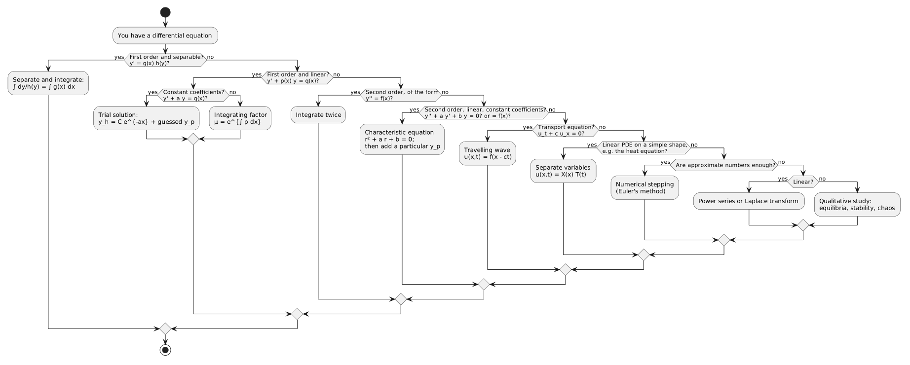
The exact methods occupy the branches on the left; most equations encountered in research fall through to the routes on the right, each treated in its own article.
A short history
The origins of differential equations coincide with those of the calculus, since the calculus supplies the language in which rates of change are expressed and inverted. Newton's laws of motion and of universal gravitation, published in the Philosophiae Naturalis Principia Mathematica (1687), are differential equations; Newton treated them by the geometrical and infinite-series methods of his fluxional calculus. Although Newton developed a notation for fluxions, the differential notation $dy/dx$ introduced by Leibniz in the 1670s proved the more enduring: it exhibits the structure of the equation directly and is the notation adopted in this article.[1]

The consolidation of these techniques into a systematic theory is due in large measure to Leonhard Euler, whose work in the middle decades of the eighteenth century established the principal exact methods. Euler showed that linear equations with constant coefficients are solved by the substitution $y=e^{rx}$, which reduces the problem to an algebraic equation, and he advanced the theory of series solutions. For equations that admitted no closed-form solution, he introduced the step-by-step numerical procedure, described above as Euler's method, that bears his name. The exact methods presented in this article derive, in large part, from his work.[1]

The theory of partial differential equations arose from the demands of eighteenth-century physics. In 1747, Jean le Rond d'Alembert derived the wave equation for the vibrating string and established that its general solution consists of two waves propagating in opposite directions. The problem of heat conduction proved more demanding, because the initial temperature distribution of a conducting body is arbitrary. In his Théorie analytique de la chaleur (1822), Joseph Fourier derived the heat equation from the physical principles of conduction and solved it by expanding the initial data into a trigonometric series. This work established separation of variables as a standard technique of mathematical physics, and the Fourier series introduced for the purpose has since become fundamental to the analysis of periodic phenomena, from acoustics to signal processing.[2]
The limits of closed-form methods became apparent towards the end of the nineteenth century, and the later history of the subject is concerned principally with equations for which elementary solutions do not exist. In his investigation of the three-body problem of celestial mechanics, Henri Poincaré demonstrated that qualitative properties of the motion, such as its equilibria, stability, and long-term behaviour, can be characterised without solving the equations, thereby founding the qualitative theory of dynamical systems. The subsequent development of electronic computing made numerical approximation, of which Euler's method is the simplest instance, a routine and general technique. The two strands converged in 1963, when Edward Lorenz, studying a simplified system of three ordinary differential equations that models atmospheric convection, established the phenomenon of deterministic chaos: although the equations are deterministic, their solutions are aperiodic and depend so sensitively on initial conditions that long-term weather prediction is not feasible in practice. These later approaches, qualitative analysis, numerical approximation, and series and transform methods, are treated in dedicated articles.[4]
References
- ↑ ↑ ↑ Tenenbaum, M. (1985). Ordinary Differential Equations (Book). In Ordinary Differential Equations (Book). Dover Publications.
- ↑ ↑ ↑ Strauss, W. A. (2008). Partial Differential Equations: An Introduction (Book). In Partial Differential Equations: An Introduction (Book). John Wiley & Sons.
- ↑ Boyce, W. E. (2012). Elementary Differential Equations and Boundary Value Problems (Book). In Elementary Differential Equations and Boundary Value Problems (Book). John Wiley & Sons.
- ↑ ↑ Strogatz, S. H. (2015). Nonlinear Dynamics and Chaos: With Applications to Physics, Biology, Chemistry, and Engineering (Book). In Nonlinear Dynamics and Chaos: With Applications to Physics, Biology, Chemistry, and Engineering (Book). Westview Press.
Further reading
- Differential equation, Wikipedia
- Differential Equation, Wolfram MathWorld
- 18.03SC Differential Equations, MIT OpenCourseWare
- Leonhard Euler, MacTutor History of Mathematics