Differential equation: Difference between revisions
Rewrite in canonical style for non-specialist readers: full worked derivations, concrete numeric examples, slope fields, and links (not duplication) to the separate articles on series, Laplace, numerical, and qualitative methods. AI-assisted (RonzzWikiCowriter) (via update-page on MediaWiki MCP Server) |
No edit summary |
||
| Line 1: | Line 1: | ||
'''A differential equation''' is an equation in which the unknown is a function, and in which the derivatives (rates of change) of that function also appear. An ordinary equation such as $x^2 = 9$ | '''A differential equation''' is an equation in which the unknown is a function, and in which the derivatives (rates of change) of that function also appear. An ordinary equation such as $x^2 = 9$ has numbers as solution; whereas a differential equation like $2y+y'=0$ has functions $y(x)$ as solution. | ||
Most laws of nature are stated as rules about how quantities change, so differential equations appear throughout science and engineering: the swinging of a pendulum, the cooling of a hot drink, the growth of a population, and the discharge of a capacitor are all described by differential equations. This article covers '''ordinary differential equations''' (ODEs), in which the unknown function depends on a single independent variable, and points to the articles that treat the more advanced solution techniques. | Most laws of nature are stated as rules about how quantities change, so differential equations appear throughout science and engineering: the swinging of a pendulum, the cooling of a hot drink, the growth of a population, and the discharge of a capacitor are all described by differential equations. This article covers '''ordinary differential equations''' (ODEs), in which the unknown function depends on a single independent variable, and points to the articles that treat the more advanced solution techniques. | ||
| Line 21: | Line 21: | ||
The solutions are therefore not one function but a whole family of parabolas $y = x^2 + C$, one for each choice of $C$, each a vertical shift of the others. This family is called the '''general solution'''. | The solutions are therefore not one function but a whole family of parabolas $y = x^2 + C$, one for each choice of $C$, each a vertical shift of the others. This family is called the '''general solution'''. | ||
How can we arrive at a '''specific solution''', i.e., one particular function of the family? An extra piece of information is required. | |||
Suppose we know when $x = 0$, $y = 3$. Substituting those numbers in we have: | |||
$$3=0^{2}+C\qquad\Longrightarrow\qquad C=3$$ | |||
$$ | Therefore | ||
$$y = x^{2} + 3$$ | |||
Such an extra condition is called an '''initial condition'''. | |||
== | == Classifying differential equations == | ||
=== Order === | === Order === | ||
| Line 44: | Line 45: | ||
where $x(t)$ is the position of a body of mass $m$ and $F$ is the net force. | where $x(t)$ is the position of a body of mass $m$ and $F$ is the net force. | ||
In general, an nth order '''ordinary differential equation''' may be solved by integrating n times. Since each integration introduces one arbitrary constant, the general solution typically contains $n$ constants. Therefore $n$ extra conditions are needed to fix them. | |||
Take a free-falling object for example. | |||
Ignoring air resistance, the only force is gravity | |||
$F_g = -mg$ | |||
By Newton's 2nd law | |||
$$m\frac{d^{2}x}{dt^{2}}=-mg\qquad\Longrightarrow\qquad\frac{d^{2}x}{dt^{2}}=-g$$ | $$m\frac{d^{2}x}{dt^{2}}=-mg\qquad\Longrightarrow\qquad\frac{d^{2}x}{dt^{2}}=-g$$ | ||
| Line 62: | Line 71: | ||
$$0=19.6-4.9\,t^{2}\qquad\Longrightarrow\qquad t=\sqrt{19.6/4.9}=2\ \text{seconds}$$ | $$0=19.6-4.9\,t^{2}\qquad\Longrightarrow\qquad t=\sqrt{19.6/4.9}=2\ \text{seconds}$$ | ||
Notice how a differential equation can predict the future: the two initial conditions fix the whole trajectory. | |||
=== | === Linearity and homogeneity === | ||
A differential equation is '''linear''' when the unknown function and its derivatives appear only to the first power and are never multiplied together (multiplying by functions of the independent variable is allowed). A | A differential equation is '''linear''' when the unknown function and its derivatives appear only to the first power and are never multiplied together (multiplying by functions of the independent variable is allowed). | ||
A linear equation can always be written as | |||
$$\frac{dy}{dx}+p(x)\,y=q(x)$$ | $$\frac{dy}{dx}+p(x)\,y=q(x)$$ | ||
Furthermore, a linear equation is known as '''homogeneous''' when $q(x)=0$. It takes the form: | |||
$$\frac{dy}{dx}+p(x)\,y=0$$ | |||
The equations | The equations | ||
| Line 74: | Line 89: | ||
$$\frac{dy}{dx}=y^{2},\qquad \frac{d^{2}\theta}{dt^{2}}+\sin\theta=0$$ | $$\frac{dy}{dx}=y^{2},\qquad \frac{d^{2}\theta}{dt^{2}}+\sin\theta=0$$ | ||
are nonlinear: the first contains the square of the unknown, the second the sine of it. | are therefore nonlinear: the first contains the square of the unknown function, the second the sine of it. | ||
Linearity and homogeneity matter because homogeneous linear equations follow the '''superposition principle'''. If $y_{1}$ and $y_{2}$ both solve a homogeneous linear equation, then any combination of thos functions $c_{1}y_{1} + c_{2}y_{2}$ solves it too. | |||
Nonlinear equations do not follow the superposition principle. If $y_{1}$ and $y_{2}$ solve $dy/dx = y^{2}$, their sum does not. | |||
In general, linear equations can be systematically solved by analytical methods, whereas most nonlinear equations cannot. | |||
=== Ordinary and partial === | === Ordinary and partial === | ||
| Line 84: | Line 103: | ||
$$\frac{\partial u}{\partial t}=\alpha\,\frac{\partial^{2}u}{\partial x^{2}}$$ | $$\frac{\partial u}{\partial t}=\alpha\,\frac{\partial^{2}u}{\partial x^{2}}$$ | ||
where the constant $\alpha$ measures how quickly heat spreads: a spot that is much warmer than its neighbours (large second derivative) warms or cools quickly | where the constant $\alpha$ measures how quickly heat spreads: a spot that is much warmer than its neighbours (large second derivative) warms or cools quickly. | ||
== Slope fields: | == Slope fields: visualising solutions == | ||
A first-order equation solved for its derivative | A first-order equation solved for its derivative has the general form | ||
{{#content:Q1581}} | {{#content:Q1581}} | ||
| Line 94: | Line 113: | ||
It assigns to every point $(x, y)$ of the plane the slope that any solution curve passing through that point must have there. Drawing a short line segment with exactly that slope at many points produces a '''direction field''' (or slope field) for the equation. | It assigns to every point $(x, y)$ of the plane the slope that any solution curve passing through that point must have there. Drawing a short line segment with exactly that slope at many points produces a '''direction field''' (or slope field) for the equation. | ||
[[File:Slope field of exponential growth.png|thumb|Direction field of $dy/dx = y$. Each short segment shows the slope that a solution must have there, and the drawn curves follow the field | [[File:Slope field of exponential growth.png|thumb|Direction field of $dy/dx = y$. Each short segment shows the slope that a solution must have there, and the drawn curves follow the field. Credit: jjbeard (public domain).]] | ||
A solution curve must be tangent to the field everywhere it passes, like a boat that is pushed by a current whose direction depends on where the boat is. The field therefore displays the whole solution family at a glance.<ref>{{#cite:Q1576}}</ref> | |||
== Solving differential equations == | |||
== | === Ordinary differential equations (ODE) === | ||
==== Linear ODE ==== | |||
Certain simple linear differential equations can be solved via '''separation of variables''' | |||
{{#content:Q1612}} | {{#content:Q1612}} | ||
For example: | |||
{{#content:Q1584}} | {{#content:Q1584}} | ||
where $k$ a constant. can be solved via separation of variables | |||
$$\frac{1}{y}\frac{dy}{dt}=k\qquad\Longrightarrow\qquad\int\frac{dy}{y}=\int k\,dt$$ | $$\frac{1}{y}\frac{dy}{dt}=k\qquad\Longrightarrow\qquad\int\frac{dy}{y}=\int k\,dt$$ | ||
Therefore | |||
$$\ln|y| = kt + C$$ | |||
Exponentiating both sides | |||
$$|y|=e^{kt+C}=e^{C}e^{kt}$$ | $$|y|=e^{kt+C}=e^{C}e^{kt}$$ | ||
Consider the initial condition $y_{0} = y(0)$ we have: | |||
{{#content:Q1585}} | {{#content:Q1585}} | ||
Notice therefore $\frac{dy}{dt}=k\,y$ describes exponential growth/decay. For $k > 0$ the quantity grows, describing a population with unlimited food, money in the bank earning steady interest, etc. ); for $k < 0$ the quantity decays, describing the decay of a radioactive substance. etc.. | |||
Another example that can be solved by the separation of variables is Newton's law of cooling: | |||
{{#content:Q1586}} | |||
{ | where $T(t)$ is the temperature of the object, $T_{a}$ the (constant) room temperature and the rate of convection $k > 0$. | ||
Separate the variables and integrate | |||
$$\int\frac{dT}{T-T_{a}}=\int -k\,dt\qquad\Longrightarrow\qquad \ln|T-T_{a}|=-kt+C$$ | $$\int\frac{dT}{T-T_{a}}=\int -k\,dt\qquad\Longrightarrow\qquad \ln|T-T_{a}|=-kt+C$$ | ||
| Line 146: | Line 163: | ||
$$|T-T_{a}|=e^{-kt+C}=e^{C}e^{-kt}$$ | $$|T-T_{a}|=e^{-kt+C}=e^{C}e^{-kt}$$ | ||
For an object hotter than the room, $T - T_{a} > 0$ | If $T > T_{a}$ the object cools; if $T < T_{a}$ it warms. | ||
For an object hotter than the room that cools, $T - T_{a} > 0$, so the absolute value can be dropped, and considering the initial condition $T(0)=T_0$ | |||
$$T(t)=T_{a}+\left(T_{0}-T_{a}\right)e^{-kt}$$ | $$T(t)=T_{a}+\left(T_{0}-T_{a}\right)e^{-kt}$$ | ||
In a sense, this is also a case of exponential decay: the temperature does not decay exponentially, but the temperature gap $T-T_a$ does. | |||
<!-- discuss other analytical methods for 1st/2nd order ODE --> | |||
=== Partial differential equations (PDE) === | |||
<!-- discuss analytical solution for simple PDEs--> | |||
== The harmonic oscillator: equations whose solutions oscillate == | == The harmonic oscillator: equations whose solutions oscillate == <!-- This should be an example, not its own section --> | ||
Some quantities do not settle towards a level but swing back and forth. Consider a mass $m$ attached to a spring. If the spring is displaced a distance $x$ from its rest position, it pulls back with a force $-kx$ proportional to the displacement (Hooke's law), where the spring constant $k$ measures how stiff the spring is. Newton's second law therefore gives | Some quantities do not settle towards a level but swing back and forth. Consider a mass $m$ attached to a spring. If the spring is displaced a distance $x$ from its rest position, it pulls back with a force $-kx$ proportional to the displacement (Hooke's law), where the spring constant $k$ measures how stiff the spring is. Newton's second law therefore gives | ||
| Line 190: | Line 209: | ||
about 4 cm on the other side of the rest position. This kind of motion, a sinusoid of fixed amplitude, is called '''simple harmonic motion''', and the oscillator equation governs not only springs but pendulums (for small swings), electric circuits, and the vibrations of molecules.<ref>{{#cite:Q1577}}</ref> | about 4 cm on the other side of the rest position. This kind of motion, a sinusoid of fixed amplitude, is called '''simple harmonic motion''', and the oscillator equation governs not only springs but pendulums (for small swings), electric circuits, and the vibrations of molecules.<ref>{{#cite:Q1577}}</ref> | ||
== | === Power series, Laplace transform, and numerical/qualitative methods === | ||
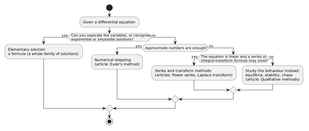
Above, we present some analytical methods to solve certain differential equations. Unfortunately, most differential equations, and almost all nonlinear ones, cannot be solved analytically by any of the methods listed above. Those complex differential equations are therefore studied in one of three ways: | |||
* | * '''Numerical approximation''' (for example, via [[Euler's method]]); | ||
* if the behaviour matters | * '''[[Qualitative methods]]''': if the behaviour of a differential equation system matters, they are studied geometrically, through its slope fields, equilibria, stability, and long-term behaviour | ||
* for special | * for certain special cases, solutions can be expressed as infinite series ([[Power series]]) or recovered by integral transforms ([[Laplace transform]]). | ||
<!-- update to reflect different analytical methods --> | |||
<uml type="uml"> | <uml type="uml"> | ||
@startuml | @startuml | ||
| Line 220: | Line 240: | ||
</uml> | </uml> | ||
The choice between | The choice between the different solution routes is part of the art of applying mathematics.<ref>{{#cite:Q1576}}</ref><ref>{{#cite:Q1578}}</ref> | ||
== A short history == | == A short history == | ||
<!-- rewrite. Less mannerism and mechanical dating, more lively --> | |||
[[File:Isaac Newton portrait.jpg|thumb|left|Isaac Newton (portrait after Godfrey Kneller, 1689). The laws of motion and of gravitation published in the ''Principia'' (1687) are differential equations. Credit: James Thronill after Godfrey Kneller (public domain).]] | [[File:Isaac Newton portrait.jpg|thumb|left|Isaac Newton (portrait after Godfrey Kneller, 1689). The laws of motion and of gravitation published in the ''Principia'' (1687) are differential equations. Credit: James Thronill after Godfrey Kneller (public domain).]] | ||
Revision as of 15:19, 5 September 2026
A differential equation is an equation in which the unknown is a function, and in which the derivatives (rates of change) of that function also appear. An ordinary equation such as $x^2 = 9$ has numbers as solution; whereas a differential equation like $2y+y'=0$ has functions $y(x)$ as solution.
Most laws of nature are stated as rules about how quantities change, so differential equations appear throughout science and engineering: the swinging of a pendulum, the cooling of a hot drink, the growth of a population, and the discharge of a capacitor are all described by differential equations. This article covers ordinary differential equations (ODEs), in which the unknown function depends on a single independent variable, and points to the articles that treat the more advanced solution techniques.
A first example: slopes and a family of solutions
Take the simplest possible differential equation. Suppose the unknown is a function $y(x)$, and all we are told about it is how it changes:
$$\frac{dy}{dx}=2x$$
Here $dy/dx$ is the slope of the graph of $y$. The equation says that whatever the solution is, its slope at the point $x$ must equal $2x$.
To solve the equation is to find every function whose slope behaves this way. Integrating both sides with respect to $x$ undoes the differentiation on the left, so
$$\int\frac{dy}{dx}\,dx=\int 2x\,dx\qquad\Longrightarrow\qquad y(x)=x^{2}+C$$
where $C$ is an arbitrary constant, because differentiating $x^2 + C$ gives $2x$ for every value of $C$:
$$\frac{d}{dx}\left(x^{2}+C\right)=2x$$
The solutions are therefore not one function but a whole family of parabolas $y = x^2 + C$, one for each choice of $C$, each a vertical shift of the others. This family is called the general solution.
How can we arrive at a specific solution, i.e., one particular function of the family? An extra piece of information is required.
Suppose we know when $x = 0$, $y = 3$. Substituting those numbers in we have:
$$3=0^{2}+C\qquad\Longrightarrow\qquad C=3$$
Therefore
$$y = x^{2} + 3$$
Such an extra condition is called an initial condition.
Classifying differential equations
Order
The order of a differential equation is the order of the highest derivative that appears in it. The equation $dy/dx = 2x$ of the previous section is first order.
Newton's second law of motion is the standard second-order example: the acceleration of a body, the second derivative of its position, is proportional to the force acting on it:
where $x(t)$ is the position of a body of mass $m$ and $F$ is the net force.
In general, an nth order ordinary differential equation may be solved by integrating n times. Since each integration introduces one arbitrary constant, the general solution typically contains $n$ constants. Therefore $n$ extra conditions are needed to fix them.
Take a free-falling object for example.
Ignoring air resistance, the only force is gravity
$F_g = -mg$
By Newton's 2nd law
$$m\frac{d^{2}x}{dt^{2}}=-mg\qquad\Longrightarrow\qquad\frac{d^{2}x}{dt^{2}}=-g$$
with $g \approx 9.8\ \mathrm{m\,s^{-2}}$ the acceleration of free fall. Integrating both sides once gives the velocity, and introduces the constant $v_{0}$, the speed at time $t = 0$:
$$\frac{dx}{dt}=-gt+v_{0}$$
Integrating again gives the height, and introduces a second constant, $x_{0}$, the height at $t = 0$:
$$x(t)=-\frac{g}{2}\,t^{2}+v_{0}t+x_{0}$$
Two conditions, the initial height and the initial velocity, are needed to fix both constants.
A concrete check: a ball dropped from rest ($v_{0} = 0$) at a height of $19.6\ \mathrm{m}$ hits the ground when $x(t) = 0$:
$$0=19.6-4.9\,t^{2}\qquad\Longrightarrow\qquad t=\sqrt{19.6/4.9}=2\ \text{seconds}$$
Notice how a differential equation can predict the future: the two initial conditions fix the whole trajectory.
Linearity and homogeneity
A differential equation is linear when the unknown function and its derivatives appear only to the first power and are never multiplied together (multiplying by functions of the independent variable is allowed).
A linear equation can always be written as
$$\frac{dy}{dx}+p(x)\,y=q(x)$$
Furthermore, a linear equation is known as homogeneous when $q(x)=0$. It takes the form:
$$\frac{dy}{dx}+p(x)\,y=0$$
The equations
$$\frac{dy}{dx}=y^{2},\qquad \frac{d^{2}\theta}{dt^{2}}+\sin\theta=0$$
are therefore nonlinear: the first contains the square of the unknown function, the second the sine of it.
Linearity and homogeneity matter because homogeneous linear equations follow the superposition principle. If $y_{1}$ and $y_{2}$ both solve a homogeneous linear equation, then any combination of thos functions $c_{1}y_{1} + c_{2}y_{2}$ solves it too.
Nonlinear equations do not follow the superposition principle. If $y_{1}$ and $y_{2}$ solve $dy/dx = y^{2}$, their sum does not.
In general, linear equations can be systematically solved by analytical methods, whereas most nonlinear equations cannot.
Ordinary and partial
An ordinary differential equation involves a function of a single independent variable, as in all the examples so far. A partial differential equation (PDE) involves a function of several independent variables, together with its partial derivatives. For example, the temperature $u(x, t)$ of a metal bar satisfies the heat equation
$$\frac{\partial u}{\partial t}=\alpha\,\frac{\partial^{2}u}{\partial x^{2}}$$
where the constant $\alpha$ measures how quickly heat spreads: a spot that is much warmer than its neighbours (large second derivative) warms or cools quickly.
Slope fields: visualising solutions
A first-order equation solved for its derivative has the general form
It assigns to every point $(x, y)$ of the plane the slope that any solution curve passing through that point must have there. Drawing a short line segment with exactly that slope at many points produces a direction field (or slope field) for the equation.

A solution curve must be tangent to the field everywhere it passes, like a boat that is pushed by a current whose direction depends on where the boat is. The field therefore displays the whole solution family at a glance.[1]
Solving differential equations
Ordinary differential equations (ODE)
Linear ODE
Certain simple linear differential equations can be solved via separation of variables
For example:
where $k$ a constant. can be solved via separation of variables
$$\frac{1}{y}\frac{dy}{dt}=k\qquad\Longrightarrow\qquad\int\frac{dy}{y}=\int k\,dt$$
Therefore
$$\ln|y| = kt + C$$
Exponentiating both sides
$$|y|=e^{kt+C}=e^{C}e^{kt}$$
Consider the initial condition $y_{0} = y(0)$ we have:
Notice therefore $\frac{dy}{dt}=k\,y$ describes exponential growth/decay. For $k > 0$ the quantity grows, describing a population with unlimited food, money in the bank earning steady interest, etc. ); for $k < 0$ the quantity decays, describing the decay of a radioactive substance. etc..
Another example that can be solved by the separation of variables is Newton's law of cooling:
where $T(t)$ is the temperature of the object, $T_{a}$ the (constant) room temperature and the rate of convection $k > 0$.
Separate the variables and integrate
$$\int\frac{dT}{T-T_{a}}=\int -k\,dt\qquad\Longrightarrow\qquad \ln|T-T_{a}|=-kt+C$$
Exponentiating both sides,
$$|T-T_{a}|=e^{-kt+C}=e^{C}e^{-kt}$$
If $T > T_{a}$ the object cools; if $T < T_{a}$ it warms.
For an object hotter than the room that cools, $T - T_{a} > 0$, so the absolute value can be dropped, and considering the initial condition $T(0)=T_0$
$$T(t)=T_{a}+\left(T_{0}-T_{a}\right)e^{-kt}$$
In a sense, this is also a case of exponential decay: the temperature does not decay exponentially, but the temperature gap $T-T_a$ does.
Partial differential equations (PDE)
The harmonic oscillator: equations whose solutions oscillate
Some quantities do not settle towards a level but swing back and forth. Consider a mass $m$ attached to a spring. If the spring is displaced a distance $x$ from its rest position, it pulls back with a force $-kx$ proportional to the displacement (Hooke's law), where the spring constant $k$ measures how stiff the spring is. Newton's second law therefore gives
$$m\frac{d^{2}x}{dt^{2}}=-kx\qquad\Longrightarrow\qquad\frac{d^{2}x}{dt^{2}}+\frac{k}{m}x=0$$
Writing $\omega_{0}^{2} = k/m$, this becomes the harmonic oscillator equation:
The equation asks for a function whose second derivative is a negative constant multiple of itself, and the sine and cosine have exactly this property. Differentiating $\cos(\omega_{0}t)$ twice brings out two factors of $\omega_{0}$ and a minus sign:
$$\frac{d}{dt}\cos(\omega_{0}t)=-\omega_{0}\sin(\omega_{0}t),\qquad \frac{d^{2}}{dt^{2}}\cos(\omega_{0}t)=-\omega_{0}^{2}\cos(\omega_{0}t)$$
so $x = \cos(\omega_{0}t)$ solves the equation, and so does $x = \sin(\omega_{0}t)$. Because the equation is linear and homogeneous, the superposition principle applies and the general solution is
$$x(t)=A\cos(\omega_{0}t)+B\sin(\omega_{0}t)$$
The two constants $A$ and $B$ are fixed by the initial displacement and the initial velocity, exactly as the order of the equation requires.

A concrete example. Take a mass of $2\ \mathrm{kg}$ on a spring with $k = 8\ \mathrm{N/m}$, so that $\omega_{0} = \sqrt{k/m} = \sqrt{4} = 2$ radians per second. Pull the mass $10\ \mathrm{cm}$ out and release it from rest: the initial velocity is zero, so $B = 0$, and $x(t) = 0.10\cos(2t)$ metres. The motion repeats after one period
$$P=\frac{2\pi}{\omega_{0}}=\pi\ \text{seconds}\approx 3.14\ \text{s}$$
so the mass returns to its starting point roughly every 3.14 seconds. One second after release, measuring angles in radians,
$$x(1)=0.10\cos(2)\approx 0.10\times(-0.416)\approx -0.042\ \text{m}$$
about 4 cm on the other side of the rest position. This kind of motion, a sinusoid of fixed amplitude, is called simple harmonic motion, and the oscillator equation governs not only springs but pendulums (for small swings), electric circuits, and the vibrations of molecules.[2]
Power series, Laplace transform, and numerical/qualitative methods
Above, we present some analytical methods to solve certain differential equations. Unfortunately, most differential equations, and almost all nonlinear ones, cannot be solved analytically by any of the methods listed above. Those complex differential equations are therefore studied in one of three ways:
- Numerical approximation (for example, via Euler's method);
- Qualitative methods: if the behaviour of a differential equation system matters, they are studied geometrically, through its slope fields, equilibria, stability, and long-term behaviour
- for certain special cases, solutions can be expressed as infinite series (Power series) or recovered by integral transforms (Laplace transform).
The choice between the different solution routes is part of the art of applying mathematics.[1][3]
A short history

Differential equations arose together with the calculus developed by Isaac Newton and Gottfried Wilhelm Leibniz in the second half of the 17th century. Newton's laws of motion, published in his Principia of 1687, are differential equations, and it is Leibniz's notation $dy/dx$, introduced in the same period, that is still used today. In the 18th century Leonhard Euler turned a collection of ad hoc tricks into a systematic theory, developing the solution of linear equations with constant coefficients, series methods, and the first numerical integration scheme, which still bears his name.[2]

Alongside the theory of ordinary equations, the physics of the 18th and 19th centuries produced the partial differential equations: Jean le Rond d'Alembert wrote down and solved the wave equation of the vibrating string in the 1740s, and Joseph Fourier derived the heat equation from the physics of conduction and solved it with trigonometric series in his Théorie analytique de la chaleur of 1822, founding Fourier analysis.[4]
Two developments of the 20th century completed the modern picture. On the one hand, numerical computing made it possible to approximate the solutions of equations that cannot be solved in formulas. On the other, the geometric ideas of Henri Poincaré, who studied the three-body problem of celestial mechanics at the end of the 19th century, grew into the qualitative theory of dynamical systems, in which equilibria, stability, and long-term behaviour are studied without solving the equations. In 1963 the meteorologist Edward Lorenz found chaotic behaviour in a simple system of three differential equations modelling atmospheric convection: although the equations were deterministic, their solutions were aperiodic and so sensitive to initial conditions that long-term weather prediction is impossible in practice.[3]
References
- ↑ ↑ Boyce, W. E. (2012). Elementary Differential Equations and Boundary Value Problems (Book). In Elementary Differential Equations and Boundary Value Problems (Book). John Wiley & Sons.
- ↑ ↑ Tenenbaum, M. (1985). Ordinary Differential Equations (Book). In Ordinary Differential Equations (Book). Dover Publications.
- ↑ ↑ Strogatz, S. H. (2015). Nonlinear Dynamics and Chaos: With Applications to Physics, Biology, Chemistry, and Engineering (Book). In Nonlinear Dynamics and Chaos: With Applications to Physics, Biology, Chemistry, and Engineering (Book). Westview Press.
- ↑ Strauss, W. A. (2008). Partial Differential Equations: An Introduction (Book). In Partial Differential Equations: An Introduction (Book). John Wiley & Sons.
Further reading
- Differential equation, Wikipedia
- Differential Equation, Wolfram MathWorld
- 18.03SC Differential Equations, MIT OpenCourseWare
- Leonhard Euler, MacTutor History of Mathematics