Differential equation: Difference between revisions
No edit summary |
AI-assisted (RonzzWikiCowriter): implement HTML-comment advice: add analytic methods for 1st/2nd order ODEs (integrating factor, characteristic equation), an analytic PDE example (heat equation by separation of variables), restructure the harmonic oscillator as an example, update the decision diagram, and rewrite the history section. (via update-page on MediaWiki MCP Server) |
||
| Line 1: | Line 1: | ||
'''A differential equation''' is an equation in which the unknown is a function, and in which the derivatives (rates of change) of that function also appear. An ordinary equation such as $x^2 = 9$ has numbers as | '''A differential equation''' is an equation in which the unknown is a function, and in which the derivatives (rates of change) of that function also appear. An ordinary equation such as $x^2 = 9$ has numbers as solutions, whereas a differential equation such as $2y+y'=0$ has functions $y(x)$ as solutions. | ||
Most laws of nature are stated as rules about how quantities change, so differential equations appear throughout science and engineering: the swinging of a pendulum, the cooling of a hot drink, the growth of a population, and the discharge of a capacitor are all described by differential equations. This article | Most laws of nature are stated as rules about how quantities change, so differential equations appear throughout science and engineering: the swinging of a pendulum, the cooling of a hot drink, the growth of a population, and the discharge of a capacitor are all described by differential equations. This article explains what a differential equation is and how equations are classified, then works through the most common exact methods of solution, each illustrated by a concrete numerical example that needs no background knowledge beyond school algebra. It treats '''ordinary differential equations''' (ODEs), in which the unknown function depends on a single independent variable, in the most detail, and gives shorter accounts of '''partial differential equations''' (PDEs) and of the numerical, series, and qualitative methods used when no exact formula exists. | ||
== A first example: slopes and a family of solutions == | == A first example: slopes and a family of solutions == | ||
| Line 21: | Line 21: | ||
The solutions are therefore not one function but a whole family of parabolas $y = x^2 + C$, one for each choice of $C$, each a vertical shift of the others. This family is called the '''general solution'''. | The solutions are therefore not one function but a whole family of parabolas $y = x^2 + C$, one for each choice of $C$, each a vertical shift of the others. This family is called the '''general solution'''. | ||
How can we arrive at a ''' | How can we arrive at a '''particular solution''', that is, one specific function of the family? An extra piece of information is required. | ||
Suppose we know when $x = 0$, $y = 3$. Substituting those numbers in we have: | Suppose we know that when $x = 0$, $y = 3$. Substituting those numbers in we have: | ||
$$3=0^{2}+C\qquad\Longrightarrow\qquad C=3$$ | $$3=0^{2}+C\qquad\Longrightarrow\qquad C=3$$ | ||
| Line 34: | Line 34: | ||
== Classifying differential equations == | == Classifying differential equations == | ||
A few labels do most of the work in deciding how to attack an equation. Three questions matter: how many derivatives appear (the ''order''), whether the unknown function enters linearly (''linearity''), and how many independent variables are involved (''ordinary or partial''). Equations that fit no convenient label are usually handled numerically or qualitatively, as described in the final section of this article. | |||
=== Order === | === Order === | ||
| Line 45: | Line 47: | ||
where $x(t)$ is the position of a body of mass $m$ and $F$ is the net force. | where $x(t)$ is the position of a body of mass $m$ and $F$ is the net force. | ||
In general, an nth order | In general, the general solution of an nth-order equation contains $n$ arbitrary constants, so $n$ extra conditions are needed to single out one particular solution. When the equation has the special form $y^{(n)}=f(x)$, the constants appear naturally, one at each of the $n$ integrations needed to undo the derivatives; the free-fall example below shows the pattern for $n = 2$. | ||
Take a free-falling object for example. | Take a free-falling object, for example. Ignoring air resistance, the only force is gravity | ||
$$F_g = -mg$$ | |||
By Newton's second law | |||
By Newton's | |||
$$m\frac{d^{2}x}{dt^{2}}=-mg\qquad\Longrightarrow\qquad\frac{d^{2}x}{dt^{2}}=-g$$ | $$m\frac{d^{2}x}{dt^{2}}=-mg\qquad\Longrightarrow\qquad\frac{d^{2}x}{dt^{2}}=-g$$ | ||
| Line 75: | Line 75: | ||
=== Linearity and homogeneity === | === Linearity and homogeneity === | ||
A differential equation is '''linear''' when the unknown function and its derivatives appear only to the first power and are never multiplied together (multiplying by functions of the independent variable is allowed). | A differential equation is '''linear''' when the unknown function and its derivatives appear only to the first power and are never multiplied together (multiplying by functions of the independent variable is allowed). A linear first-order equation can always be written as | ||
A linear equation can always be written as | |||
$$\frac{dy}{dx}+p(x)\,y=q(x)$$ | $$\frac{dy}{dx}+p(x)\,y=q(x)$$ | ||
Furthermore, a linear equation is | Furthermore, a linear equation is called '''homogeneous''' when $q(x)=0$; it then takes the form | ||
$$\frac{dy}{dx}+p(x)\,y=0$$ | $$\frac{dy}{dx}+p(x)\,y=0$$ | ||
| Line 91: | Line 89: | ||
are therefore nonlinear: the first contains the square of the unknown function, the second the sine of it. | are therefore nonlinear: the first contains the square of the unknown function, the second the sine of it. | ||
Linearity and homogeneity matter because homogeneous linear equations | Linearity and homogeneity matter because homogeneous linear equations obey the '''superposition principle'''. If $y_{1}$ and $y_{2}$ both solve a homogeneous linear equation, then any combination $c_{1}y_{1} + c_{2}y_{2}$ of those functions solves it too. This is why solutions of linear equations can be added together, a property used repeatedly later in this article (for example, to build the solution of the heat equation from simple building blocks). | ||
Nonlinear equations do not | Nonlinear equations do not obey the superposition principle. If $y_{1}$ and $y_{2}$ solve $dy/dx = y^{2}$, their sum does not. | ||
In general, linear equations can be systematically | In general, linear equations can be solved systematically, whereas most nonlinear equations cannot; the last section of this article describes what is done with those. | ||
=== Ordinary and partial === | === Ordinary and partial === | ||
An '''ordinary differential equation''' involves a function of a single independent variable, as in all the examples so far. A '''partial differential equation''' (PDE) involves a function of several independent variables, together with its partial derivatives. For example, the temperature $u(x, t)$ of a metal bar satisfies the heat equation | An '''ordinary differential equation''' involves a function of a single independent variable, as in all the examples so far. A '''partial differential equation''' (PDE) involves a function of several independent variables, together with its partial derivatives. For example, the temperature $u(x, t)$ of a metal bar, which depends on the position $x$ along the bar and on the time $t$, satisfies the '''heat equation''' | ||
{{#content:Q1590}} | |||
where the constant $\alpha$ measures how quickly heat spreads: a spot that is much warmer than its neighbours (large second derivative) warms or cools quickly. | where the constant $\alpha$ measures how quickly heat spreads: a spot that is much warmer than its neighbours (large second derivative $\partial^2 u/\partial x^2$) warms or cools quickly. | ||
== Slope fields: visualising solutions == | == Slope fields: visualising solutions == | ||
| Line 115: | Line 113: | ||
[[File:Slope field of exponential growth.png|thumb|Direction field of $dy/dx = y$. Each short segment shows the slope that a solution must have there, and the drawn curves follow the field. Credit: jjbeard (public domain).]] | [[File:Slope field of exponential growth.png|thumb|Direction field of $dy/dx = y$. Each short segment shows the slope that a solution must have there, and the drawn curves follow the field. Credit: jjbeard (public domain).]] | ||
A solution curve must be tangent to the field everywhere it passes, like a boat | A solution curve must be tangent to the field everywhere it passes, like a boat pushed by a current whose direction depends on where the boat is. The field therefore displays the whole solution family at a glance.<ref>{{#cite:Q1576}}</ref> Numerical methods, such as [[Euler's method]], work by following such arrows step by step: from a starting point, read the slope of the arrow there, take a small step in that direction, read the new arrow, and repeat. | ||
== Solving differential equations == | == Solving differential equations == | ||
There is no single recipe that solves every differential equation. The practical approach is to recognise which family an equation belongs to, then apply that family's method. The subsections below work through the families that appear most often, each stated in general and then illustrated with numbers; the last subsection collects the routes taken when none of these formulas applies. | |||
=== | === Separation of variables === | ||
A first-order equation is '''separable''' when the right-hand side splits into a factor that depends only on $x$ and a factor that depends only on $y$: | |||
{{#content:Q1612}} | {{#content:Q1612}} | ||
The arrow shows the whole method: divide both sides by $h(y)$ and integrate, so that all the $y$'s are on one side and all the $x$'s on the other. The two worked examples below carry this out completely, and both lead to the same conclusion: quantities whose rate of change is proportional to their own size change exponentially. | |||
==== Worked example: exponential growth and decay ==== | |||
Many quantities change at a rate proportional to their own size. A population with unlimited food grows faster the larger it is, money in a bank earns interest in proportion to the balance, and the number of radioactive atoms left decreases in proportion to how many remain. Writing the constant of proportionality as $k$, | |||
{{#content:Q1584}} | {{#content:Q1584}} | ||
where $k$ a constant. | where $k$ is a constant. To solve it, divide both sides by $y$ and integrate both sides with respect to $t$: | ||
$$\frac{1}{y}\frac{dy}{dt}=k\qquad\Longrightarrow\qquad\int\frac{dy}{y}=\int k\,dt$$ | $$\frac{1}{y}\frac{dy}{dt}=k\qquad\Longrightarrow\qquad\int\frac{dy}{y}=\int k\,dt$$ | ||
The left-hand integral is $\ln|y|$, so | |||
$$\ln|y| = kt + C$$ | $$\ln|y| = kt + C$$ | ||
Exponentiating both sides | Exponentiating both sides (raising $e$ to the power of each side) removes the logarithm: | ||
$$|y|=e^{kt+C}=e^{C}e^{kt}$$ | $$|y|=e^{kt+C}=e^{C}e^{kt}$$ | ||
The sign of $y$ never changes, so the absolute value can be dropped by absorbing the sign into the constant. Writing $y_{0}$ for the value at $t = 0$, we obtain | |||
{{#content:Q1585}} | {{#content:Q1585}} | ||
With numbers: suppose €1000 is deposited in an account paying 5% per year with interest added continuously, so $k = 0.05$ per year and $y_{0} = 1000$. The balance is $y(t) = 1000\,e^{0.05t}$, and after 10 years | |||
$$y(10)=1000\,e^{0.05\times 10}=1000\,e^{0.5}\approx 1648.7$$ | |||
so the deposit has grown to about €1649. To find when it doubles, set $y(t) = 2000$ and solve: | |||
$$1000\,e^{0.05t}=2000\qquad\Longrightarrow\qquad e^{0.05t}=2\qquad\Longrightarrow\qquad t=\frac{\ln 2}{0.05}\approx 13.9\ \text{years}$$ | |||
For $k < 0$ the same formula describes decay rather than growth. Radioactive substances are usually described by their '''half-life''', the time in which half the atoms decay; setting $y(t)=y_{0}/2$ gives $t_{1/2}=(\ln 2)/(-k)$. | |||
==== Worked example: Newton's law of cooling ==== | |||
A hot object left in a cooler room cools at a rate proportional to how much hotter it is than the room. This is Newton's law of cooling, | |||
{{#content:Q1586}} | {{#content:Q1586}} | ||
where $T(t)$ is the temperature of the object, $T_{a}$ the | where $T(t)$ is the temperature of the object, $T_{a}$ is the constant room temperature, and the positive constant $k$ measures how easily heat escapes. | ||
Separating variables means bringing everything that involves $T$ to the left: | |||
$$\int\frac{dT}{T-T_{a}}=\int -k\,dt | $$\frac{1}{T-T_{a}}\frac{dT}{dt}=-k\qquad\Longrightarrow\qquad\int\frac{dT}{T-T_{a}}=\int -k\,dt$$ | ||
Integrating both sides gives | |||
$$\ln|T-T_{a}|=-kt+C$$ | |||
Exponentiating both sides, | Exponentiating both sides, | ||
| Line 163: | Line 179: | ||
$$|T-T_{a}|=e^{-kt+C}=e^{C}e^{-kt}$$ | $$|T-T_{a}|=e^{-kt+C}=e^{C}e^{-kt}$$ | ||
The difference $T - T_{a}$ keeps its sign: positive while the object cools, negative while it warms towards a warmer room. Absorbing the sign into the constant and fixing it with the initial temperature $T(0)=T_{0}$, we obtain | |||
$$T(t)=T_{a}+\left(T_{0}-T_{a}\right)e^{-kt}$$ | |||
So the temperature does not decay exponentially, but the temperature gap $T - T_{a}$ does. | |||
With numbers: suppose a drink at $80\,^{\circ}\mathrm{C}$ is left in a room at $20\,^{\circ}\mathrm{C}$, and measurement shows $k = 0.1$ per minute. Then | |||
$$T(t)=20+\left(80-20\right)e^{-0.1t}=20+60\,e^{-0.1t}$$ | |||
The gap starts at $60\,^{\circ}\mathrm{C}$ and shrinks by the factor $e^{-0.1t}$ each minute; it halves every $(\ln 2)/0.1 \approx 6.9$ minutes. To find when the drink reaches $40\,^{\circ}\mathrm{C}$, put $T(t)=40$: | |||
$$40=20+60\,e^{-0.1t}\qquad\Longrightarrow\qquad e^{-0.1t}=\frac{1}{3}\qquad\Longrightarrow\qquad t=10\ln 3\approx 11\ \text{minutes}$$ | |||
In about 11 minutes the drink is two-thirds of the way from $80\,^{\circ}\mathrm{C}$ down to the room's $20\,^{\circ}\mathrm{C}$, and it approaches the room temperature without ever quite reaching it.<ref>{{#cite:Q1576}}</ref> | |||
=== First-order linear equations: the integrating factor === | |||
The two equations just solved are separable as well as linear. Many first-order equations, however, are linear but not separable, and for those there is a general method based on the '''integrating factor'''. | |||
Recall from the classification section that a linear first-order equation has the form | |||
$$\frac{dy}{dx}+p(x)\,y=q(x)$$ | |||
The idea is to multiply both sides by a function $\mu(x)$, chosen so that the left-hand side becomes the derivative of a single product $\mu(x)\,y$, which can then be integrated in one stroke. Expanding the product rule, | |||
$$\frac{d}{dx}\bigl(\mu(x)\,y\bigr)=\mu\,\frac{dy}{dx}+\frac{d\mu}{dx}\,y$$ | |||
Multiplying the equation by $\mu$ would give $\mu\,\frac{dy}{dx}+\mu p\,y$ on the left. For the two to agree, the coefficient of $y$ must match, so $\mu$ must satisfy $\mu' = p\,\mu$. This is itself a separable equation, solved exactly as in the previous subsection: | |||
$$\frac{d\mu}{dx}=p(x)\,\mu\qquad\Longrightarrow\qquad\frac{d\mu}{\mu}=p(x)\,dx\qquad\Longrightarrow\qquad\ln\mu=\int p(x)\,dx\qquad\Longrightarrow\qquad\mu(x)=e^{\int p(x)\,dx}$$ | |||
(any constant of integration may be taken as zero, since multiplying $\mu$ by a constant changes nothing). Multiplying the original equation by this $\mu(x)$, | |||
{{#content:Q1613}} | |||
and because the left-hand side is now a single derivative, both sides integrate immediately: | |||
$$\mu(x)\,y=\int \mu(x)\,q(x)\,dx + C$$ | |||
Worked example. Solve $y' + y = e^{-x}$. Here $p = 1$, so the integrating factor is | |||
$$\mu=e^{\int 1\,dx}=e^{x}$$ | |||
Multiplying both sides by $e^{x}$, | |||
$$e^{x}y'+e^{x}y=e^{x}e^{-x}=1$$ | |||
The left-hand side is $(e^{x}y)'$, so | |||
$$\left(e^{x}y\right)'=1\qquad\Longrightarrow\qquad e^{x}y=x+C\qquad\Longrightarrow\qquad y=(x+C)e^{-x}$$ | |||
{{#content:Q1607}} | |||
An initial condition fixes the constant: if $y(0)=2$, then $2=(0+C)e^{0}$, so $C=2$ and $y=(x+2)e^{-x}$.<ref>{{#cite:Q1576}}</ref><ref>{{#cite:Q1577}}</ref> | |||
=== Constant-coefficient linear equations of order two === | |||
The methods so far solve first-order equations. The most important second-order family is the linear equation with constant coefficients, | |||
$$ | $$y''+a\,y'+b\,y=0$$ | ||
which models systems pulled back towards a resting state: a mass on a spring, a pendulum swinging through small angles, and an electric circuit containing a capacitor and an inductor. The key idea is to try an exponential solution $y=e^{rx}$, because the derivative of an exponential is again a multiple of itself, so substituting turns the differential equation into an ordinary algebraic equation: | |||
{{#content:Q1644}} | |||
To see where the arrow comes from, substitute $y=e^{rx}$ together with $y'=re^{rx}$ and $y''=r^{2}e^{rx}$ into the equation: | |||
$$r^{2}e^{rx}+a\,r\,e^{rx}+b\,e^{rx}=\left(r^{2}+a\,r+b\right)e^{rx}=0$$ | |||
Since $e^{rx}$ is never zero, divide both sides by it: | |||
$$r^{2}+a\,r+b=0$$ | |||
This is the '''characteristic equation'''. It is an ordinary quadratic equation, and the form of the solution depends on the kind of roots it has: | |||
* '''Two distinct real roots''', $r_{1} \neq r_{2}$: the general solution is $y=C_{1}e^{r_{1}x}+C_{2}e^{r_{2}x}$, a sum of two exponentials. | |||
* '''One repeated real root''', $r$: the general solution is $y=\left(C_{1}+C_{2}x\right)e^{rx}$; the extra factor $x$ supplies the second arbitrary constant. | |||
* '''A complex conjugate pair''', $r=\alpha \pm i\beta$: the general solution is $y=e^{\alpha x}\left(C_{1}\cos\beta x + C_{2}\sin\beta x\right)$, which oscillates, growing or fading in size according to the sign of $\alpha$. | |||
A quick numerical example of the first case: solve $y''-3y'+2y=0$. Substituting $y=e^{rx}$ gives $r^{2}-3r+2=0=(r-1)(r-2)$, so the roots are $1$ and $2$, and | |||
{{#content:Q1608}} | |||
Each term works, as can be checked directly: for $y=e^{x}$, one has $y''-3y'+2y=(1-3+2)e^{x}=0$, and similarly for $e^{2x}$. | |||
== | ==== Example: the harmonic oscillator (a mass on a spring) ==== | ||
Some quantities do not settle towards a level but swing back and forth. Consider a mass $m$ attached to a spring. If the spring is displaced a distance $x$ from its rest position, it pulls back with a force $-kx$ proportional to the displacement (Hooke's law), where the spring constant $k$ measures how stiff the spring is. Newton's second law therefore gives | Some quantities do not settle towards a level but swing back and forth. The complex-root case above is not an exotic exception: it is exactly what happens for the most common oscillating system of all. Consider a mass $m$ attached to a spring. If the spring is displaced a distance $x$ from its rest position, it pulls back with a force $-kx$ proportional to the displacement (Hooke's law), where the spring constant $k$ measures how stiff the spring is. Newton's second law therefore gives | ||
$$m\frac{d^{2}x}{dt^{2}}=-kx\qquad\Longrightarrow\qquad\frac{d^{2}x}{dt^{2}}+\frac{k}{m}x=0$$ | $$m\frac{d^{2}x}{dt^{2}}=-kx\qquad\Longrightarrow\qquad\frac{d^{2}x}{dt^{2}}+\frac{k}{m}x=0$$ | ||
| Line 187: | Line 275: | ||
{{#content:Q1588}} | {{#content:Q1588}} | ||
The equation asks for a function whose second derivative is a negative constant multiple of itself, and the sine and cosine have exactly this property. Differentiating $\cos(\omega_{0}t)$ twice brings out two factors of $\omega_{0}$ and a minus sign: | Its characteristic equation is $r^{2}+\omega_{0}^{2}=0$, with the purely imaginary roots $r=\pm i\omega_{0}$: this is the complex-conjugate case above with $\alpha=0$ and $\beta=\omega_{0}$. The equation asks for a function whose second derivative is a negative constant multiple of itself, and the sine and cosine have exactly this property. Differentiating $\cos(\omega_{0}t)$ twice brings out two factors of $\omega_{0}$ and a minus sign: | ||
$$\frac{d}{dt}\cos(\omega_{0}t)=-\omega_{0}\sin(\omega_{0}t),\qquad \frac{d^{2}}{dt^{2}}\cos(\omega_{0}t)=-\omega_{0}^{2}\cos(\omega_{0}t)$$ | $$\frac{d}{dt}\cos(\omega_{0}t)=-\omega_{0}\sin(\omega_{0}t),\qquad \frac{d^{2}}{dt^{2}}\cos(\omega_{0}t)=-\omega_{0}^{2}\cos(\omega_{0}t)$$ | ||
| Line 209: | Line 297: | ||
about 4 cm on the other side of the rest position. This kind of motion, a sinusoid of fixed amplitude, is called '''simple harmonic motion''', and the oscillator equation governs not only springs but pendulums (for small swings), electric circuits, and the vibrations of molecules.<ref>{{#cite:Q1577}}</ref> | about 4 cm on the other side of the rest position. This kind of motion, a sinusoid of fixed amplitude, is called '''simple harmonic motion''', and the oscillator equation governs not only springs but pendulums (for small swings), electric circuits, and the vibrations of molecules.<ref>{{#cite:Q1577}}</ref> | ||
=== | === Partial differential equations: separating variables in the heat equation === | ||
Exact formulas for partial differential equations exist only for a few simple, usually linear, problems, but these are precisely the problems at the heart of physics and engineering. The standard technique is again separation of variables, but now the variables to be separated are the independent variables themselves, here the position $x$ and the time $t$. | |||
Return to the metal bar of the classification section, this time of length $L$ with its sides insulated, so that heat flows only along the bar, and with both ends held at temperature $0$. Its temperature $u(x,t)$ satisfies the heat equation, reproduced here: | |||
$$\frac{\partial u}{\partial t}=\alpha\,\frac{\partial^{2}u}{\partial x^{2}}$$ | |||
Separation of variables looks for a solution that splits into a product of a function of $x$ alone and a function of $t$ alone: | |||
$$u(x,t)=X(x)\,T(t)$$ | |||
Substituting into the heat equation gives $X\,T'=\alpha\,X''\,T$. Divide both sides by $\alpha X T$: | |||
{{#content:Q1622}} | |||
The left-hand side now depends only on $t$ and the right-hand side only on $x$. Since $x$ and $t$ can vary independently, the only way two functions of different variables can be equal for all $x$ and $t$ is that both sides equal the same constant, written above as $-\lambda$. This splits the partial differential equation into two ordinary ones: | |||
* $T'=-\alpha\lambda\,T$: exponential decay, the growth equation of this article with $k=-\alpha\lambda<0$, giving $T=e^{-\alpha\lambda t}$; | |||
* $X''=-\lambda X$: the function whose second derivative is a negative constant multiple of itself, giving sines and cosines of $\sqrt{\lambda}\,x$. | |||
The ends of the bar are held at temperature $0$, so $u(0,t)=u(L,t)=0$, which forces $X(0)=X(L)=0$. The condition $X(0)=0$ removes the cosine, and $X(L)=0$ forces $\sin(\sqrt{\lambda}\,L)=0$, so $\sqrt{\lambda}\,L=n\pi$ for a positive whole number $n$. Thus only the special values $\lambda=(n\pi/L)^{2}$ are allowed, each giving one mode | |||
$$u_{n}(x,t)=\sin\left(\frac{n\pi x}{L}\right)e^{-\alpha(n\pi/L)^{2}t}$$ | |||
* '''Numerical approximation''' | a half-wave, or several half-waves, of a sine curve that sinks towards zero as heat leaks out of the ends. Because the heat equation is linear and homogeneous, superposition applies: any sum of modes is again a solution, and the general solution is | ||
* '''[[Qualitative methods]]''': | |||
* for | {{#content:Q1611}} | ||
The numbers $b_{n}$ are fixed by the initial temperature profile $u(x,0)$ at $t=0$; writing an arbitrary initial profile as such a sum of sine waves is exactly what Fourier's sine series does. | |||
Two features are worth noticing. First, every mode decays exponentially, so the bar does not oscillate: heat spreads and the temperature evens out. Second, modes with more wiggles decay faster, because their rate $-\alpha(n\pi/L)^{2}$ is larger in magnitude, so after a short time only the $n=1$ mode, one smooth half-sine across the whole bar, is left. | |||
A concrete check with numbers: take a one-metre iron bar (iron's thermal diffusivity is $\alpha \approx 2.3\times10^{-5}\ \mathrm{m^{2}\,s^{-1}}$) whose initial temperature is $u(x,0)=100\sin(\pi x/L)$, that is, $0\,^{\circ}\mathrm{C}$ at the ends and $100\,^{\circ}\mathrm{C}$ in the middle. Only the $n=1$ mode is present, so | |||
$$u(x,t)=100\,\sin\left(\frac{\pi x}{L}\right)e^{-\alpha\pi^{2}t/L^{2}}$$ | |||
With $L=1\ \mathrm{m}$, the decay rate is $\alpha\pi^{2}\approx 2.3\times10^{-5}\times9.87\approx 2.3\times10^{-4}$ per second. At the centre of the bar, where the sine equals $1$, | |||
$$u\!\left(\tfrac{1}{2},t\right)=100\,e^{-2.3\times10^{-4}\,t}$$ | |||
After one hour ($t=3600\ \mathrm{s}$) the exponent is $2.3\times10^{-4}\times3600\approx0.82$, so the centre has cooled to $100\,e^{-0.82}\approx44\,^{\circ}\mathrm{C}$, and it reaches $50\,^{\circ}\mathrm{C}$ after $t=(\ln 2)/(2.3\times10^{-4})\approx 3050\ \mathrm{s}$, about 51 minutes. The heat has flowed out through the ends, exactly the phenomenon Fourier set out to describe.<ref>{{#cite:Q1579}}</ref> | |||
=== When no formula is possible: numerical, series, and qualitative methods === | |||
The families above, separable and linear with convenient coefficients, cover a great many practical equations, but they are a small minority of all differential equations. There is no guarantee that a given equation, especially a nonlinear one, has a solution expressible in terms of the familiar functions at all. Such equations are studied in one of three ways: | |||
* '''Numerical approximation''', when numbers are what is needed: [[Euler's method]] steps forward along the slope field, replacing the exact solution by a polygonal path, and its refinements underlie most computer simulations; | |||
* '''[[Qualitative methods]]''', when behaviour matters more than numbers: the solutions are studied through the slope field, equilibria, stability, and long-term behaviour, without ever writing a formula; | |||
* '''Series and integral transforms''', for special but important cases: when an equation is linear, a solution can sometimes be written as an infinite series ([[Power series]]) or recovered from an algebraic equation by the [[Laplace transform]]. | |||
Choosing between these routes is part of the art of applying mathematics, and the diagram below summarises the decision process of this whole article.<ref>{{#cite:Q1576}}</ref><ref>{{#cite:Q1578}}</ref> | |||
<uml type="uml"> | <uml type="uml"> | ||
@startuml | @startuml | ||
skinparam monochrome true | skinparam monochrome true | ||
start | start | ||
: | :You have a differential equation; | ||
if ( | if (Is it first order and separable?\ny' = g(x) h(y)?) then (yes) | ||
: | :Separate and integrate:\n∫ dy/h(y) = ∫ g(x) dx; | ||
else (no) | else (no) | ||
if ( | if (Is it first order and linear?\ny' + p(x) y = q(x)?) then (yes) | ||
: | :Multiply by the integrating factor\nμ = e^{∫ p dx}, then integrate; | ||
else (no) | else (no) | ||
if ( | if (Is it second order, linear, with constant coefficients?\ny'' + a y' + b y = 0?) then (yes) | ||
: | :Solve the characteristic equation\nr² + a r + b = 0; | ||
else (no) | else (no) | ||
:Study | if (Is it a linear PDE on a simple\nshape, e.g. the heat equation?) then (yes) | ||
:Separate the variables:\nu(x,t) = X(x) T(t); | |||
else (no) | |||
if (Are approximate numbers enough?) then (yes) | |||
:Step forward numerically\n(article: Euler's method); | |||
else (no) | |||
if (Is the equation linear?) then (yes) | |||
:Power series or Laplace transform\n(articles: Power series, Laplace transform); | |||
else (no) | |||
:Study behaviour without formulas:\nequilibria, stability, chaos\n(article: Qualitative methods); | |||
endif | |||
endif | |||
endif | |||
endif | endif | ||
endif | endif | ||
| Line 240: | Line 384: | ||
</uml> | </uml> | ||
As the diagram shows, the exact methods occupy only the first few branches; most equations encountered in research are handled by the routes at the bottom of the diagram, each of which has its own article. | |||
== A short history == | == A short history == | ||
Differential equations are as old as the calculus itself, because the calculus is the mathematics of change: the laws of physics say how quantities change, and predicting the future means undoing those changes. When Newton published his laws of motion and of gravitation in the ''Principia'' in 1687, the equations he needed were differential equations, and he solved them by geometry and by infinite series. Newton had his own notation for rates of change, but it was Leibniz's $dy/dx$, first written in the 1670s, that survived: it displays the whole equation on the page, and it is the notation used throughout this article.<ref>{{#cite:Q1577}}</ref> | |||
[[File:Isaac Newton portrait.jpg|thumb|left|Isaac Newton (portrait after Godfrey Kneller, 1689). The laws of motion and of gravitation published in the ''Principia'' (1687) are differential equations. Credit: James Thronill after Godfrey Kneller (public domain).]] | [[File:Isaac Newton portrait.jpg|thumb|left|Isaac Newton (portrait after Godfrey Kneller, 1689). The laws of motion and of gravitation published in the ''Principia'' (1687) are differential equations. Credit: James Thronill after Godfrey Kneller (public domain).]] | ||
The scattered tricks of the early calculus became a subject when [[Person:Leonhard Euler|Leonhard Euler]] took them up in the middle decades of the 18th century. He recognised that a linear equation with constant coefficients is solved by substituting $y=e^{rx}$, turning calculus into algebra; he developed series solutions; and, for equations that resisted formulas, he invented the step-by-step numerical scheme, described in this article, that still bears his name. Most of the exact methods above descend from his work.<ref>{{#cite:Q1577}}</ref> | |||
[[File:Leonhard Euler portrait.jpg|thumb|Leonhard Euler (portrait by Jakob Emanuel Handmann, 1753) | [[File:Leonhard Euler portrait.jpg|thumb|Leonhard Euler (portrait by Jakob Emanuel Handmann, 1753). Credit: Jakob Emanuel Handmann (public domain).]] | ||
Meanwhile physics began asking for equations with more than one independent variable. A plucked string takes a shape that depends on position along the string and on time, and in 1747 [[Person:Jean le Rond d'Alembert|Jean le Rond d'Alembert]] wrote down the wave equation for it and solved it, showing that its solutions are two waves travelling in opposite directions. Heat conduction posed a subtler problem, because the initial temperature of a bar can have any shape at all. [[Person:Joseph Fourier|Joseph Fourier]] derived the heat equation from the physics of conduction and, to solve it, had to express an arbitrary initial profile as a sum of sine ripples. His ''Théorie analytique de la chaleur'' of 1822 turned separation of variables into a cornerstone of applied mathematics, and the Fourier series invented for the purpose now appears wherever signals are analysed, from acoustics to image compression.<ref>{{#cite:Q1579}}</ref> | |||
The exact formulas, however, have their limits, and the history of the subject since the late 19th century is largely the story of what to do when no formula exists. Studying the three-body problem of celestial mechanics, [[Person:Henri Poincaré|Henri Poincaré]] realised that the shape of the motion can be understood without solving the equations, founding the qualitative theory of dynamical systems. The electronic computer then made the numerical route routine: approximate the solution step by step, as Euler's method does, refining the steps until the error is acceptable. The two strands met in 1963, when the meteorologist [[Person:Edward Lorenz|Edward Lorenz]] found that a simple system of three differential equations, meant to model atmospheric convection, behaved chaotically: the equations were deterministic, yet their solutions were aperiodic and so sensitive to initial conditions that long-term weather prediction is impossible in practice. Each of these later routes, qualitative study, numerical stepping, series, and transforms, is the subject of its own article.<ref>{{#cite:Q1578}}</ref> | |||
== References == | == References == | ||
Revision as of 18:40, 5 September 2026
A differential equation is an equation in which the unknown is a function, and in which the derivatives (rates of change) of that function also appear. An ordinary equation such as $x^2 = 9$ has numbers as solutions, whereas a differential equation such as $2y+y'=0$ has functions $y(x)$ as solutions.
Most laws of nature are stated as rules about how quantities change, so differential equations appear throughout science and engineering: the swinging of a pendulum, the cooling of a hot drink, the growth of a population, and the discharge of a capacitor are all described by differential equations. This article explains what a differential equation is and how equations are classified, then works through the most common exact methods of solution, each illustrated by a concrete numerical example that needs no background knowledge beyond school algebra. It treats ordinary differential equations (ODEs), in which the unknown function depends on a single independent variable, in the most detail, and gives shorter accounts of partial differential equations (PDEs) and of the numerical, series, and qualitative methods used when no exact formula exists.
A first example: slopes and a family of solutions
Take the simplest possible differential equation. Suppose the unknown is a function $y(x)$, and all we are told about it is how it changes:
$$\frac{dy}{dx}=2x$$
Here $dy/dx$ is the slope of the graph of $y$. The equation says that whatever the solution is, its slope at the point $x$ must equal $2x$.
To solve the equation is to find every function whose slope behaves this way. Integrating both sides with respect to $x$ undoes the differentiation on the left, so
$$\int\frac{dy}{dx}\,dx=\int 2x\,dx\qquad\Longrightarrow\qquad y(x)=x^{2}+C$$
where $C$ is an arbitrary constant, because differentiating $x^2 + C$ gives $2x$ for every value of $C$:
$$\frac{d}{dx}\left(x^{2}+C\right)=2x$$
The solutions are therefore not one function but a whole family of parabolas $y = x^2 + C$, one for each choice of $C$, each a vertical shift of the others. This family is called the general solution.
How can we arrive at a particular solution, that is, one specific function of the family? An extra piece of information is required.
Suppose we know that when $x = 0$, $y = 3$. Substituting those numbers in we have:
$$3=0^{2}+C\qquad\Longrightarrow\qquad C=3$$
Therefore
$$y = x^{2} + 3$$
Such an extra condition is called an initial condition.
Classifying differential equations
A few labels do most of the work in deciding how to attack an equation. Three questions matter: how many derivatives appear (the order), whether the unknown function enters linearly (linearity), and how many independent variables are involved (ordinary or partial). Equations that fit no convenient label are usually handled numerically or qualitatively, as described in the final section of this article.
Order
The order of a differential equation is the order of the highest derivative that appears in it. The equation $dy/dx = 2x$ of the previous section is first order.
Newton's second law of motion is the standard second-order example: the acceleration of a body, the second derivative of its position, is proportional to the force acting on it:
where $x(t)$ is the position of a body of mass $m$ and $F$ is the net force.
In general, the general solution of an nth-order equation contains $n$ arbitrary constants, so $n$ extra conditions are needed to single out one particular solution. When the equation has the special form $y^{(n)}=f(x)$, the constants appear naturally, one at each of the $n$ integrations needed to undo the derivatives; the free-fall example below shows the pattern for $n = 2$.
Take a free-falling object, for example. Ignoring air resistance, the only force is gravity
$$F_g = -mg$$
By Newton's second law
$$m\frac{d^{2}x}{dt^{2}}=-mg\qquad\Longrightarrow\qquad\frac{d^{2}x}{dt^{2}}=-g$$
with $g \approx 9.8\ \mathrm{m\,s^{-2}}$ the acceleration of free fall. Integrating both sides once gives the velocity, and introduces the constant $v_{0}$, the speed at time $t = 0$:
$$\frac{dx}{dt}=-gt+v_{0}$$
Integrating again gives the height, and introduces a second constant, $x_{0}$, the height at $t = 0$:
$$x(t)=-\frac{g}{2}\,t^{2}+v_{0}t+x_{0}$$
Two conditions, the initial height and the initial velocity, are needed to fix both constants.
A concrete check: a ball dropped from rest ($v_{0} = 0$) at a height of $19.6\ \mathrm{m}$ hits the ground when $x(t) = 0$:
$$0=19.6-4.9\,t^{2}\qquad\Longrightarrow\qquad t=\sqrt{19.6/4.9}=2\ \text{seconds}$$
Notice how a differential equation can predict the future: the two initial conditions fix the whole trajectory.
Linearity and homogeneity
A differential equation is linear when the unknown function and its derivatives appear only to the first power and are never multiplied together (multiplying by functions of the independent variable is allowed). A linear first-order equation can always be written as
$$\frac{dy}{dx}+p(x)\,y=q(x)$$
Furthermore, a linear equation is called homogeneous when $q(x)=0$; it then takes the form
$$\frac{dy}{dx}+p(x)\,y=0$$
The equations
$$\frac{dy}{dx}=y^{2},\qquad \frac{d^{2}\theta}{dt^{2}}+\sin\theta=0$$
are therefore nonlinear: the first contains the square of the unknown function, the second the sine of it.
Linearity and homogeneity matter because homogeneous linear equations obey the superposition principle. If $y_{1}$ and $y_{2}$ both solve a homogeneous linear equation, then any combination $c_{1}y_{1} + c_{2}y_{2}$ of those functions solves it too. This is why solutions of linear equations can be added together, a property used repeatedly later in this article (for example, to build the solution of the heat equation from simple building blocks).
Nonlinear equations do not obey the superposition principle. If $y_{1}$ and $y_{2}$ solve $dy/dx = y^{2}$, their sum does not.
In general, linear equations can be solved systematically, whereas most nonlinear equations cannot; the last section of this article describes what is done with those.
Ordinary and partial
An ordinary differential equation involves a function of a single independent variable, as in all the examples so far. A partial differential equation (PDE) involves a function of several independent variables, together with its partial derivatives. For example, the temperature $u(x, t)$ of a metal bar, which depends on the position $x$ along the bar and on the time $t$, satisfies the heat equation
where the constant $\alpha$ measures how quickly heat spreads: a spot that is much warmer than its neighbours (large second derivative $\partial^2 u/\partial x^2$) warms or cools quickly.
Slope fields: visualising solutions
A first-order equation solved for its derivative has the general form
It assigns to every point $(x, y)$ of the plane the slope that any solution curve passing through that point must have there. Drawing a short line segment with exactly that slope at many points produces a direction field (or slope field) for the equation.

A solution curve must be tangent to the field everywhere it passes, like a boat pushed by a current whose direction depends on where the boat is. The field therefore displays the whole solution family at a glance.[1] Numerical methods, such as Euler's method, work by following such arrows step by step: from a starting point, read the slope of the arrow there, take a small step in that direction, read the new arrow, and repeat.
Solving differential equations
There is no single recipe that solves every differential equation. The practical approach is to recognise which family an equation belongs to, then apply that family's method. The subsections below work through the families that appear most often, each stated in general and then illustrated with numbers; the last subsection collects the routes taken when none of these formulas applies.
Separation of variables
A first-order equation is separable when the right-hand side splits into a factor that depends only on $x$ and a factor that depends only on $y$:
The arrow shows the whole method: divide both sides by $h(y)$ and integrate, so that all the $y$'s are on one side and all the $x$'s on the other. The two worked examples below carry this out completely, and both lead to the same conclusion: quantities whose rate of change is proportional to their own size change exponentially.
Worked example: exponential growth and decay
Many quantities change at a rate proportional to their own size. A population with unlimited food grows faster the larger it is, money in a bank earns interest in proportion to the balance, and the number of radioactive atoms left decreases in proportion to how many remain. Writing the constant of proportionality as $k$,
where $k$ is a constant. To solve it, divide both sides by $y$ and integrate both sides with respect to $t$:
$$\frac{1}{y}\frac{dy}{dt}=k\qquad\Longrightarrow\qquad\int\frac{dy}{y}=\int k\,dt$$
The left-hand integral is $\ln|y|$, so
$$\ln|y| = kt + C$$
Exponentiating both sides (raising $e$ to the power of each side) removes the logarithm:
$$|y|=e^{kt+C}=e^{C}e^{kt}$$
The sign of $y$ never changes, so the absolute value can be dropped by absorbing the sign into the constant. Writing $y_{0}$ for the value at $t = 0$, we obtain
With numbers: suppose €1000 is deposited in an account paying 5% per year with interest added continuously, so $k = 0.05$ per year and $y_{0} = 1000$. The balance is $y(t) = 1000\,e^{0.05t}$, and after 10 years
$$y(10)=1000\,e^{0.05\times 10}=1000\,e^{0.5}\approx 1648.7$$
so the deposit has grown to about €1649. To find when it doubles, set $y(t) = 2000$ and solve:
$$1000\,e^{0.05t}=2000\qquad\Longrightarrow\qquad e^{0.05t}=2\qquad\Longrightarrow\qquad t=\frac{\ln 2}{0.05}\approx 13.9\ \text{years}$$
For $k < 0$ the same formula describes decay rather than growth. Radioactive substances are usually described by their half-life, the time in which half the atoms decay; setting $y(t)=y_{0}/2$ gives $t_{1/2}=(\ln 2)/(-k)$.
Worked example: Newton's law of cooling
A hot object left in a cooler room cools at a rate proportional to how much hotter it is than the room. This is Newton's law of cooling,
where $T(t)$ is the temperature of the object, $T_{a}$ is the constant room temperature, and the positive constant $k$ measures how easily heat escapes.
Separating variables means bringing everything that involves $T$ to the left:
$$\frac{1}{T-T_{a}}\frac{dT}{dt}=-k\qquad\Longrightarrow\qquad\int\frac{dT}{T-T_{a}}=\int -k\,dt$$
Integrating both sides gives
$$\ln|T-T_{a}|=-kt+C$$
Exponentiating both sides,
$$|T-T_{a}|=e^{-kt+C}=e^{C}e^{-kt}$$
The difference $T - T_{a}$ keeps its sign: positive while the object cools, negative while it warms towards a warmer room. Absorbing the sign into the constant and fixing it with the initial temperature $T(0)=T_{0}$, we obtain
$$T(t)=T_{a}+\left(T_{0}-T_{a}\right)e^{-kt}$$
So the temperature does not decay exponentially, but the temperature gap $T - T_{a}$ does.
With numbers: suppose a drink at $80\,^{\circ}\mathrm{C}$ is left in a room at $20\,^{\circ}\mathrm{C}$, and measurement shows $k = 0.1$ per minute. Then
$$T(t)=20+\left(80-20\right)e^{-0.1t}=20+60\,e^{-0.1t}$$
The gap starts at $60\,^{\circ}\mathrm{C}$ and shrinks by the factor $e^{-0.1t}$ each minute; it halves every $(\ln 2)/0.1 \approx 6.9$ minutes. To find when the drink reaches $40\,^{\circ}\mathrm{C}$, put $T(t)=40$:
$$40=20+60\,e^{-0.1t}\qquad\Longrightarrow\qquad e^{-0.1t}=\frac{1}{3}\qquad\Longrightarrow\qquad t=10\ln 3\approx 11\ \text{minutes}$$
In about 11 minutes the drink is two-thirds of the way from $80\,^{\circ}\mathrm{C}$ down to the room's $20\,^{\circ}\mathrm{C}$, and it approaches the room temperature without ever quite reaching it.[1]
First-order linear equations: the integrating factor
The two equations just solved are separable as well as linear. Many first-order equations, however, are linear but not separable, and for those there is a general method based on the integrating factor.
Recall from the classification section that a linear first-order equation has the form
$$\frac{dy}{dx}+p(x)\,y=q(x)$$
The idea is to multiply both sides by a function $\mu(x)$, chosen so that the left-hand side becomes the derivative of a single product $\mu(x)\,y$, which can then be integrated in one stroke. Expanding the product rule,
$$\frac{d}{dx}\bigl(\mu(x)\,y\bigr)=\mu\,\frac{dy}{dx}+\frac{d\mu}{dx}\,y$$
Multiplying the equation by $\mu$ would give $\mu\,\frac{dy}{dx}+\mu p\,y$ on the left. For the two to agree, the coefficient of $y$ must match, so $\mu$ must satisfy $\mu' = p\,\mu$. This is itself a separable equation, solved exactly as in the previous subsection:
$$\frac{d\mu}{dx}=p(x)\,\mu\qquad\Longrightarrow\qquad\frac{d\mu}{\mu}=p(x)\,dx\qquad\Longrightarrow\qquad\ln\mu=\int p(x)\,dx\qquad\Longrightarrow\qquad\mu(x)=e^{\int p(x)\,dx}$$
(any constant of integration may be taken as zero, since multiplying $\mu$ by a constant changes nothing). Multiplying the original equation by this $\mu(x)$,
and because the left-hand side is now a single derivative, both sides integrate immediately:
$$\mu(x)\,y=\int \mu(x)\,q(x)\,dx + C$$
Worked example. Solve $y' + y = e^{-x}$. Here $p = 1$, so the integrating factor is
$$\mu=e^{\int 1\,dx}=e^{x}$$
Multiplying both sides by $e^{x}$,
$$e^{x}y'+e^{x}y=e^{x}e^{-x}=1$$
The left-hand side is $(e^{x}y)'$, so
$$\left(e^{x}y\right)'=1\qquad\Longrightarrow\qquad e^{x}y=x+C\qquad\Longrightarrow\qquad y=(x+C)e^{-x}$$
An initial condition fixes the constant: if $y(0)=2$, then $2=(0+C)e^{0}$, so $C=2$ and $y=(x+2)e^{-x}$.[1][2]
Constant-coefficient linear equations of order two
The methods so far solve first-order equations. The most important second-order family is the linear equation with constant coefficients,
$$y''+a\,y'+b\,y=0$$
which models systems pulled back towards a resting state: a mass on a spring, a pendulum swinging through small angles, and an electric circuit containing a capacitor and an inductor. The key idea is to try an exponential solution $y=e^{rx}$, because the derivative of an exponential is again a multiple of itself, so substituting turns the differential equation into an ordinary algebraic equation:
To see where the arrow comes from, substitute $y=e^{rx}$ together with $y'=re^{rx}$ and $y''=r^{2}e^{rx}$ into the equation:
$$r^{2}e^{rx}+a\,r\,e^{rx}+b\,e^{rx}=\left(r^{2}+a\,r+b\right)e^{rx}=0$$
Since $e^{rx}$ is never zero, divide both sides by it:
$$r^{2}+a\,r+b=0$$
This is the characteristic equation. It is an ordinary quadratic equation, and the form of the solution depends on the kind of roots it has:
- Two distinct real roots, $r_{1} \neq r_{2}$: the general solution is $y=C_{1}e^{r_{1}x}+C_{2}e^{r_{2}x}$, a sum of two exponentials.
- One repeated real root, $r$: the general solution is $y=\left(C_{1}+C_{2}x\right)e^{rx}$; the extra factor $x$ supplies the second arbitrary constant.
- A complex conjugate pair, $r=\alpha \pm i\beta$: the general solution is $y=e^{\alpha x}\left(C_{1}\cos\beta x + C_{2}\sin\beta x\right)$, which oscillates, growing or fading in size according to the sign of $\alpha$.
A quick numerical example of the first case: solve $y''-3y'+2y=0$. Substituting $y=e^{rx}$ gives $r^{2}-3r+2=0=(r-1)(r-2)$, so the roots are $1$ and $2$, and
Each term works, as can be checked directly: for $y=e^{x}$, one has $y''-3y'+2y=(1-3+2)e^{x}=0$, and similarly for $e^{2x}$.
Example: the harmonic oscillator (a mass on a spring)
Some quantities do not settle towards a level but swing back and forth. The complex-root case above is not an exotic exception: it is exactly what happens for the most common oscillating system of all. Consider a mass $m$ attached to a spring. If the spring is displaced a distance $x$ from its rest position, it pulls back with a force $-kx$ proportional to the displacement (Hooke's law), where the spring constant $k$ measures how stiff the spring is. Newton's second law therefore gives
$$m\frac{d^{2}x}{dt^{2}}=-kx\qquad\Longrightarrow\qquad\frac{d^{2}x}{dt^{2}}+\frac{k}{m}x=0$$
Writing $\omega_{0}^{2} = k/m$, this becomes the harmonic oscillator equation:
Its characteristic equation is $r^{2}+\omega_{0}^{2}=0$, with the purely imaginary roots $r=\pm i\omega_{0}$: this is the complex-conjugate case above with $\alpha=0$ and $\beta=\omega_{0}$. The equation asks for a function whose second derivative is a negative constant multiple of itself, and the sine and cosine have exactly this property. Differentiating $\cos(\omega_{0}t)$ twice brings out two factors of $\omega_{0}$ and a minus sign:
$$\frac{d}{dt}\cos(\omega_{0}t)=-\omega_{0}\sin(\omega_{0}t),\qquad \frac{d^{2}}{dt^{2}}\cos(\omega_{0}t)=-\omega_{0}^{2}\cos(\omega_{0}t)$$
so $x = \cos(\omega_{0}t)$ solves the equation, and so does $x = \sin(\omega_{0}t)$. Because the equation is linear and homogeneous, the superposition principle applies and the general solution is
$$x(t)=A\cos(\omega_{0}t)+B\sin(\omega_{0}t)$$
The two constants $A$ and $B$ are fixed by the initial displacement and the initial velocity, exactly as the order of the equation requires.

A concrete example. Take a mass of $2\ \mathrm{kg}$ on a spring with $k = 8\ \mathrm{N/m}$, so that $\omega_{0} = \sqrt{k/m} = \sqrt{4} = 2$ radians per second. Pull the mass $10\ \mathrm{cm}$ out and release it from rest: the initial velocity is zero, so $B = 0$, and $x(t) = 0.10\cos(2t)$ metres. The motion repeats after one period
$$P=\frac{2\pi}{\omega_{0}}=\pi\ \text{seconds}\approx 3.14\ \text{s}$$
so the mass returns to its starting point roughly every 3.14 seconds. One second after release, measuring angles in radians,
$$x(1)=0.10\cos(2)\approx 0.10\times(-0.416)\approx -0.042\ \text{m}$$
about 4 cm on the other side of the rest position. This kind of motion, a sinusoid of fixed amplitude, is called simple harmonic motion, and the oscillator equation governs not only springs but pendulums (for small swings), electric circuits, and the vibrations of molecules.[2]
Partial differential equations: separating variables in the heat equation
Exact formulas for partial differential equations exist only for a few simple, usually linear, problems, but these are precisely the problems at the heart of physics and engineering. The standard technique is again separation of variables, but now the variables to be separated are the independent variables themselves, here the position $x$ and the time $t$.
Return to the metal bar of the classification section, this time of length $L$ with its sides insulated, so that heat flows only along the bar, and with both ends held at temperature $0$. Its temperature $u(x,t)$ satisfies the heat equation, reproduced here:
$$\frac{\partial u}{\partial t}=\alpha\,\frac{\partial^{2}u}{\partial x^{2}}$$
Separation of variables looks for a solution that splits into a product of a function of $x$ alone and a function of $t$ alone:
$$u(x,t)=X(x)\,T(t)$$
Substituting into the heat equation gives $X\,T'=\alpha\,X''\,T$. Divide both sides by $\alpha X T$:
The left-hand side now depends only on $t$ and the right-hand side only on $x$. Since $x$ and $t$ can vary independently, the only way two functions of different variables can be equal for all $x$ and $t$ is that both sides equal the same constant, written above as $-\lambda$. This splits the partial differential equation into two ordinary ones:
- $T'=-\alpha\lambda\,T$: exponential decay, the growth equation of this article with $k=-\alpha\lambda<0$, giving $T=e^{-\alpha\lambda t}$;
- $X''=-\lambda X$: the function whose second derivative is a negative constant multiple of itself, giving sines and cosines of $\sqrt{\lambda}\,x$.
The ends of the bar are held at temperature $0$, so $u(0,t)=u(L,t)=0$, which forces $X(0)=X(L)=0$. The condition $X(0)=0$ removes the cosine, and $X(L)=0$ forces $\sin(\sqrt{\lambda}\,L)=0$, so $\sqrt{\lambda}\,L=n\pi$ for a positive whole number $n$. Thus only the special values $\lambda=(n\pi/L)^{2}$ are allowed, each giving one mode
$$u_{n}(x,t)=\sin\left(\frac{n\pi x}{L}\right)e^{-\alpha(n\pi/L)^{2}t}$$
a half-wave, or several half-waves, of a sine curve that sinks towards zero as heat leaks out of the ends. Because the heat equation is linear and homogeneous, superposition applies: any sum of modes is again a solution, and the general solution is
The numbers $b_{n}$ are fixed by the initial temperature profile $u(x,0)$ at $t=0$; writing an arbitrary initial profile as such a sum of sine waves is exactly what Fourier's sine series does.
Two features are worth noticing. First, every mode decays exponentially, so the bar does not oscillate: heat spreads and the temperature evens out. Second, modes with more wiggles decay faster, because their rate $-\alpha(n\pi/L)^{2}$ is larger in magnitude, so after a short time only the $n=1$ mode, one smooth half-sine across the whole bar, is left.
A concrete check with numbers: take a one-metre iron bar (iron's thermal diffusivity is $\alpha \approx 2.3\times10^{-5}\ \mathrm{m^{2}\,s^{-1}}$) whose initial temperature is $u(x,0)=100\sin(\pi x/L)$, that is, $0\,^{\circ}\mathrm{C}$ at the ends and $100\,^{\circ}\mathrm{C}$ in the middle. Only the $n=1$ mode is present, so
$$u(x,t)=100\,\sin\left(\frac{\pi x}{L}\right)e^{-\alpha\pi^{2}t/L^{2}}$$
With $L=1\ \mathrm{m}$, the decay rate is $\alpha\pi^{2}\approx 2.3\times10^{-5}\times9.87\approx 2.3\times10^{-4}$ per second. At the centre of the bar, where the sine equals $1$,
$$u\!\left(\tfrac{1}{2},t\right)=100\,e^{-2.3\times10^{-4}\,t}$$
After one hour ($t=3600\ \mathrm{s}$) the exponent is $2.3\times10^{-4}\times3600\approx0.82$, so the centre has cooled to $100\,e^{-0.82}\approx44\,^{\circ}\mathrm{C}$, and it reaches $50\,^{\circ}\mathrm{C}$ after $t=(\ln 2)/(2.3\times10^{-4})\approx 3050\ \mathrm{s}$, about 51 minutes. The heat has flowed out through the ends, exactly the phenomenon Fourier set out to describe.[3]
When no formula is possible: numerical, series, and qualitative methods
The families above, separable and linear with convenient coefficients, cover a great many practical equations, but they are a small minority of all differential equations. There is no guarantee that a given equation, especially a nonlinear one, has a solution expressible in terms of the familiar functions at all. Such equations are studied in one of three ways:
- Numerical approximation, when numbers are what is needed: Euler's method steps forward along the slope field, replacing the exact solution by a polygonal path, and its refinements underlie most computer simulations;
- Qualitative methods, when behaviour matters more than numbers: the solutions are studied through the slope field, equilibria, stability, and long-term behaviour, without ever writing a formula;
- Series and integral transforms, for special but important cases: when an equation is linear, a solution can sometimes be written as an infinite series (Power series) or recovered from an algebraic equation by the Laplace transform.
Choosing between these routes is part of the art of applying mathematics, and the diagram below summarises the decision process of this whole article.[1][4]
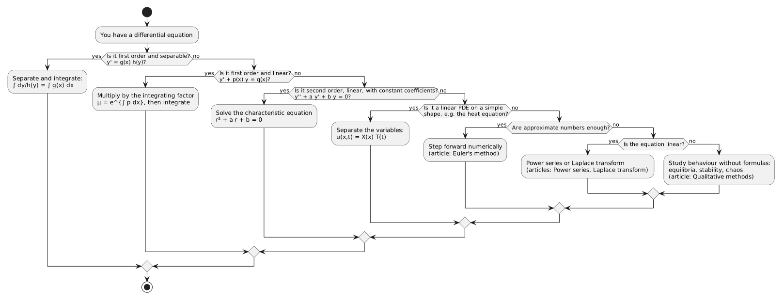
As the diagram shows, the exact methods occupy only the first few branches; most equations encountered in research are handled by the routes at the bottom of the diagram, each of which has its own article.
A short history
Differential equations are as old as the calculus itself, because the calculus is the mathematics of change: the laws of physics say how quantities change, and predicting the future means undoing those changes. When Newton published his laws of motion and of gravitation in the Principia in 1687, the equations he needed were differential equations, and he solved them by geometry and by infinite series. Newton had his own notation for rates of change, but it was Leibniz's $dy/dx$, first written in the 1670s, that survived: it displays the whole equation on the page, and it is the notation used throughout this article.[2]

The scattered tricks of the early calculus became a subject when Leonhard Euler took them up in the middle decades of the 18th century. He recognised that a linear equation with constant coefficients is solved by substituting $y=e^{rx}$, turning calculus into algebra; he developed series solutions; and, for equations that resisted formulas, he invented the step-by-step numerical scheme, described in this article, that still bears his name. Most of the exact methods above descend from his work.[2]

Meanwhile physics began asking for equations with more than one independent variable. A plucked string takes a shape that depends on position along the string and on time, and in 1747 Jean le Rond d'Alembert wrote down the wave equation for it and solved it, showing that its solutions are two waves travelling in opposite directions. Heat conduction posed a subtler problem, because the initial temperature of a bar can have any shape at all. Joseph Fourier derived the heat equation from the physics of conduction and, to solve it, had to express an arbitrary initial profile as a sum of sine ripples. His Théorie analytique de la chaleur of 1822 turned separation of variables into a cornerstone of applied mathematics, and the Fourier series invented for the purpose now appears wherever signals are analysed, from acoustics to image compression.[3]
The exact formulas, however, have their limits, and the history of the subject since the late 19th century is largely the story of what to do when no formula exists. Studying the three-body problem of celestial mechanics, Henri Poincaré realised that the shape of the motion can be understood without solving the equations, founding the qualitative theory of dynamical systems. The electronic computer then made the numerical route routine: approximate the solution step by step, as Euler's method does, refining the steps until the error is acceptable. The two strands met in 1963, when the meteorologist Edward Lorenz found that a simple system of three differential equations, meant to model atmospheric convection, behaved chaotically: the equations were deterministic, yet their solutions were aperiodic and so sensitive to initial conditions that long-term weather prediction is impossible in practice. Each of these later routes, qualitative study, numerical stepping, series, and transforms, is the subject of its own article.[4]
References
- ↑ ↑ ↑ ↑ Boyce, W. E. (2012). Elementary Differential Equations and Boundary Value Problems (Book). In Elementary Differential Equations and Boundary Value Problems (Book). John Wiley & Sons.
- ↑ ↑ ↑ ↑ Tenenbaum, M. (1985). Ordinary Differential Equations (Book). In Ordinary Differential Equations (Book). Dover Publications.
- ↑ ↑ Strauss, W. A. (2008). Partial Differential Equations: An Introduction (Book). In Partial Differential Equations: An Introduction (Book). John Wiley & Sons.
- ↑ ↑ Strogatz, S. H. (2015). Nonlinear Dynamics and Chaos: With Applications to Physics, Biology, Chemistry, and Engineering (Book). In Nonlinear Dynamics and Chaos: With Applications to Physics, Biology, Chemistry, and Engineering (Book). Westview Press.
Further reading
- Differential equation, Wikipedia
- Differential Equation, Wolfram MathWorld
- 18.03SC Differential Equations, MIT OpenCourseWare
- Leonhard Euler, MacTutor History of Mathematics