Differential equation: Difference between revisions
AI-assisted (RonzzWikiCowriter): implement HTML-comment advice: add analytic methods for 1st/2nd order ODEs (integrating factor, characteristic equation), an analytic PDE example (heat equation by separation of variables), restructure the harmonic oscillator as an example, update the decision diagram, and rewrite the history section. (via update-page on MediaWiki MCP Server) |
AI-assisted (RonzzWikiCowriter): condense the article — cut prose commentary, let the derivations and worked examples carry the explanation; keep all semantic embeds, images, diagram and citations. (via update-page on MediaWiki MCP Server) |
||
| Line 1: | Line 1: | ||
'''A differential equation''' is an equation | '''A differential equation''' is an equation whose unknown is a function and which also involves that function's derivatives (rates of change). Where an ordinary equation such as $x^2=9$ is solved by numbers, a differential equation such as $y'+2y=0$ is solved by functions $y(x)$. Laws of nature state how quantities change, so differential equations describe pendulums, cooling drinks, growing populations, and discharging capacitors. This article covers the standard exact solution methods, each with a worked numerical example, and the numerical, series, and qualitative routes used when no exact formula exists. It treats '''ordinary differential equations''' (one independent variable) and, briefly, '''partial differential equations''' (several). | ||
== A first example: slopes and a family of solutions == | == A first example: slopes and a family of solutions == | ||
The simplest differential equation prescribes the slope of a function $y(x)$: | |||
$$\frac{dy}{dx}=2x$$ | $$\frac{dy}{dx}=2x$$ | ||
Integration inverts differentiation, so integrating both sides gives | |||
$$\int\frac{dy}{dx}\,dx=\int 2x\,dx\qquad\Longrightarrow\qquad y(x)=x^{2}+C$$ | $$\int\frac{dy}{dx}\,dx=\int 2x\,dx\qquad\Longrightarrow\qquad y(x)=x^{2}+C$$ | ||
Every $C$ works, since $\frac{d}{dx}\left(x^2+C\right)=2x$; the solutions form the parabola family $y=x^2+C$, the '''general solution'''. | |||
An extra condition picks out one member. If $y(0)=3$, then | |||
$$y = x^ | $$3=0^2+C\qquad\Longrightarrow\qquad C=3\qquad\Longrightarrow\qquad y=x^2+3$$ | ||
Such | Such a prescribed value is an '''initial condition'''. | ||
== Classifying differential equations == | == Classifying differential equations == | ||
Three features decide how to solve an equation: its '''order''', its '''linearity''', and how many independent variables it involves. | |||
=== Order === | === Order === | ||
The | The order is the order of the highest derivative present. $dy/dx=2x$ is first order; Newton's second law, | ||
Newton's second law | |||
{{#content:Q1583}} | {{#content:Q1583}} | ||
is second order ($x(t)$ position of mass $m$, $F$ net force). An nth-order equation has $n$ arbitrary constants in its general solution, fixed by $n$ conditions, one constant appearing at each integration. Free fall shows the pattern: with only gravity $F_g=-mg$, Newton's law gives | |||
$$x | $$m\frac{d^{2}x}{dt^{2}}=-mg\qquad\Longrightarrow\qquad\frac{d^{2}x}{dt^{2}}=-g\qquad(g\approx 9.8\ \mathrm{m\,s^{-2}})$$ | ||
Integrate once (constant $v_0$, the speed at $t=0$), then again (constant $x_0$, the height at $t=0$): | |||
$$\frac{dx}{dt}=-gt+v_{0}\qquad\Longrightarrow\qquad x(t)=-\frac{g}{2}t^{2}+v_{0}t+x_{0}$$ | |||
$ | Two initial conditions are needed. A ball dropped from rest at height $19.6\ \mathrm{m}$ hits the ground ($x=0$) when | ||
$$0=19.6-4.9\,t^{2}\qquad\Longrightarrow\qquad t=\sqrt{19.6/4.9}=2\ \text{s}$$ | |||
=== Linearity and homogeneity === | === Linearity and homogeneity === | ||
An equation is '''linear''' when the unknown and its derivatives appear only to the first power and never multiplied together. A linear first-order equation can always be written | |||
$$\frac{dy}{dx}+p(x)\,y=q(x)$$ | $$\frac{dy}{dx}+p(x)\,y=q(x)$$ | ||
and is '''homogeneous''' when $q(x)=0$. The equations $dy/dx=y^2$ and $d^2\theta/dt^2+\sin\theta=0$ are nonlinear (square of $y$; sine of $\theta$). | |||
The equations | |||
$ | |||
are | |||
If $y_1,y_2$ solve a homogeneous linear equation, so does $c_1y_1+c_2y_2$ (the '''superposition principle'''). Nonlinear equations lack this property. Superposition underlies every linear method below. | |||
=== Ordinary and partial === | === Ordinary and partial === | ||
An '''ordinary differential equation''' | An '''ordinary differential equation''' (ODE) has one independent variable. A '''partial differential equation''' (PDE) has several, with partial derivatives; for example the temperature $u(x,t)$ of an insulated metal bar obeys the heat equation | ||
{{#content:Q1590}} | {{#content:Q1590}} | ||
where | where $\alpha$ is the thermal diffusivity. The equation says a spot cools fastest where the temperature profile is most curved ($\partial^2u/\partial x^2$ large). | ||
== Slope fields | == Slope fields == | ||
A first-order equation | A first-order equation can be written | ||
{{#content:Q1581}} | {{#content:Q1581}} | ||
assigning to each point $(x,y)$ the slope $f(x,y)$ a solution must have there. Drawing short segments of that slope gives a '''direction field'''; solution curves run tangent to it. | |||
[[File:Slope field of exponential growth.png|thumb|Direction field of $dy/dx = y$ | [[File:Slope field of exponential growth.png|thumb|Direction field of $dy/dx=y$. Credit: jjbeard (public domain).]] | ||
Numerical methods such as [[Euler's method]] follow the field: read the slope, step a short distance along it, repeat.<ref>{{#cite:Q1576}}</ref> | |||
== Solving differential equations == | == Solving differential equations == | ||
=== Separation of variables === | === Separation of variables === | ||
A first-order equation is '''separable''' when the right-hand side | A first-order equation is '''separable''' when the right-hand side factors into a function of $x$ times a function of $y$: | ||
{{#content:Q1612}} | {{#content:Q1612}} | ||
Divide by $h(y)$ and integrate; all $y$'s land on one side, all $x$'s on the other. | |||
==== | ==== Exponential growth and decay ==== | ||
When a quantity changes at a rate proportional to its own size, | |||
{{#content:Q1584}} | {{#content:Q1584}} | ||
divide by $y$ and integrate: | |||
$$|y|= | $$\int\frac{dy}{y}=\int k\,dt\qquad\Longrightarrow\qquad \ln|y|=kt+C$$ | ||
Exponentiating, $|y|=e^C e^{kt}$; the sign of $y$ never changes, so absorbing it into the constant and writing $y(0)=y_0$, | |||
{{#content:Q1585}} | {{#content:Q1585}} | ||
With numbers: | With numbers: €1000 at 5% interest compounded continuously ($k=0.05\ \text{yr}^{-1}$) gives $y(t)=1000\,e^{0.05t}$, and | ||
$$1000\,e^{0. | $$y(10)=1000\,e^{0.5}\approx 1648.7$$ | ||
For $k < 0$ the same | Doubling time: $1000\,e^{0.05t}=2000\Rightarrow t=\ln 2/0.05\approx 13.9$ years. For $k<0$ the same solution describes decay; the '''half-life''' $y=y_0/2$ is $t_{1/2}=(\ln 2)/(-k)$. | ||
==== | ==== Newton's law of cooling ==== | ||
A | A body hotter than its surroundings cools at a rate proportional to the temperature gap: | ||
{{#content:Q1586}} | {{#content:Q1586}} | ||
Separate and integrate: | |||
$$\int\frac{dT}{T-T_a}=\int-k\,dt\qquad\Longrightarrow\qquad \ln|T-T_a|=-kt+C$$ | |||
Exponentiating and folding the (constant-sign) factor $T-T_a$ into the constant, with $T(0)=T_0$: | |||
$$T(t)= | $$T(t)=T_a+(T_0-T_a)e^{-kt}$$ | ||
The gap | The gap $T-T_a$ decays exponentially, not $T$ itself. Example: a drink at $80\,^{\circ}\mathrm{C}$ in a $20\,^{\circ}\mathrm{C}$ room, $k=0.1\ \text{min}^{-1}$: | ||
$$ | $$T(t)=20+60\,e^{-0.1t}$$ | ||
Reaches $40\,^{\circ}\mathrm{C}$ when $20+60e^{-0.1t}=40$, i.e. $t=10\ln 3\approx 11$ min.<ref>{{#cite:Q1576}}</ref> | |||
=== First-order linear equations: the integrating factor === | === First-order linear equations: the integrating factor === | ||
For $y'+p(x)y=q(x)$ that is not separable, multiply by $\mu(x)$ chosen so the left side is a single derivative $(\mu y)'$. The product rule gives $(\mu y)'=\mu y'+\mu' y$, while multiplying the equation by $\mu$ gives $\mu y'+\mu p\,y$; matching coefficients requires $\mu'=p\mu$, whose solution is | |||
$$ | $$\mu(x)=e^{\int p(x)\,dx}$$ | ||
Multiplying the equation by $\mu$, | |||
{{#content:Q1613}} | {{#content:Q1613}} | ||
so both sides integrate directly: | |||
$$ | $$\mu(x)\,y=\int\mu(x)\,q(x)\,dx+C$$ | ||
Example: $y'+y=e^{-x}$. Here $p=1$, $\mu=e^x$, and | |||
$$\ | $$e^x y'+e^x y=1\qquad\Longrightarrow\qquad (e^x y)'=1\qquad\Longrightarrow\qquad e^x y=x+C\qquad\Longrightarrow\qquad y=(x+C)e^{-x}$$ | ||
{{#content:Q1607}} | {{#content:Q1607}} | ||
The condition $y(0)=2$ gives $C=2$.<ref>{{#cite:Q1576}}</ref><ref>{{#cite:Q1577}}</ref> | |||
=== Constant-coefficient linear equations of order two === | === Constant-coefficient linear equations of order two === | ||
The | The equation $y''+a\,y'+b\,y=0$ (constant coefficients) models a mass on a spring, a small-angle pendulum, and an RLC circuit. It is solved by trying an exponential $y=e^{rx}$, since $y'=re^{rx}$ and $y''=r^2e^{rx}$: | ||
{{#content:Q1644}} | {{#content:Q1644}} | ||
Substitution turns the equation into algebra: $(r^2+ar+b)e^{rx}=0$, and $e^{rx}\neq 0$, so | |||
$ | |||
$$r^ | $$r^2+ar+b=0$$ | ||
This is the '''characteristic equation''' | This is the '''characteristic equation'''; its roots determine the solution: | ||
* | * distinct real roots $r_1\neq r_2$: $y=C_1e^{r_1x}+C_2e^{r_2x}$; | ||
* | * one repeated root $r$: $y=(C_1+C_2x)e^{rx}$; | ||
* | * complex pair $r=\alpha\pm i\beta$: $y=e^{\alpha x}(C_1\cos\beta x+C_2\sin\beta x)$. | ||
Example ($y''-3y'+2y=0$): $r^2-3r+2=(r-1)(r-2)$, so | |||
{{#content:Q1608}} | {{#content:Q1608}} | ||
Each term | Each term checks: for $y=e^x$, $y''-3y'+2y=(1-3+2)e^x=0$. | ||
==== | ==== The harmonic oscillator (a mass on a spring) ==== | ||
A mass displaced $x$ from rest is pulled back by $-kx$ (Hooke's law), so Newton's second law gives | |||
$$m\frac{d^ | $$m\frac{d^2x}{dt^2}=-kx\qquad\Longrightarrow\qquad x''+\frac{k}{m}x=0$$ | ||
With $\omega_0^2=k/m$ this is the '''harmonic oscillator equation''' | |||
{{#content:Q1588}} | {{#content:Q1588}} | ||
Its characteristic equation | Its characteristic equation $r^2+\omega_0^2=0$ has roots $\pm i\omega_0$, the complex case above ($\alpha=0$). Since $\frac{d^2}{dt^2}\cos\omega_0 t=-\omega_0^2\cos\omega_0 t$, and likewise for sine, superposition gives | ||
$$x(t)=A\cos | $$x(t)=A\cos\omega_0 t+B\sin\omega_0 t$$ | ||
with $A,B$ fixed by the initial position and velocity. | |||
[[File:Simple harmonic motion animation.gif|thumb|A mass on a spring | [[File:Simple harmonic motion animation.gif|thumb|A mass on a spring: the harmonic oscillator solution is a sinusoid of fixed amplitude. Credit: Evil saltine (public domain).]] | ||
Example: $m=2\ \mathrm{kg}$, $k=8\ \mathrm{N/m}$, so $\omega_0=\sqrt{8/2}=2\ \text{rad/s}$. Pulled $10\ \mathrm{cm}$ out and released from rest, $B=0$ and $x(t)=0.10\cos 2t$ metres. The period is | |||
$$P=\frac{2\pi}{\ | $$P=\frac{2\pi}{\omega_0}=\pi\approx 3.14\ \text{s}$$ | ||
and after one second | |||
$$x(1)=0.10\cos | $$x(1)=0.10\cos 2\approx 0.10(-0.416)\approx -0.042\ \text{m}$$ | ||
Such fixed-amplitude sinusoidal motion is '''simple harmonic motion'''.<ref>{{#cite:Q1577}}</ref> | |||
=== Partial differential equations: separating variables in the heat equation === | === Partial differential equations: separating variables in the heat equation === | ||
Solve the heat equation on a bar of length $L$, insulated sides, ends held at $0$: | |||
$$\frac{\partial u}{\partial t}=\alpha\frac{\partial^2u}{\partial x^2}$$ | |||
$ | Seek a product solution $u(x,t)=X(x)T(t)$. Substitution gives $XT'=\alpha X''T$; dividing by $\alpha XT$, | ||
{{#content:Q1622}} | |||
The left side depends only on $t$, the right only on $x$, so both equal one constant, $-\lambda$. This yields two ODEs, | |||
$$T'=-\alpha\lambda T\qquad\Longrightarrow\qquad T=e^{-\alpha\lambda t}$$ | |||
$$X''=-\lambda X\qquad\Longrightarrow\qquad X=A\cos(\sqrt{\lambda}\,x)+B\sin(\sqrt{\lambda}\,x)$$ | |||
The | The end conditions $u(0,t)=u(L,t)=0$ force $X(0)=X(L)=0$: hence $A=0$ and $\sin(\sqrt\lambda\,L)=0$, so $\sqrt\lambda\,L=n\pi$, $n=1,2,\dots$ Each allowed $\lambda=(n\pi/L)^2$ gives one mode | ||
$$ | $$u_n(x,t)=\sin\frac{n\pi x}{L}\,e^{-\alpha(n\pi/L)^2t}$$ | ||
The equation is linear and homogeneous, so superposition applies, and the general solution is | |||
{{#content:Q1611}} | {{#content:Q1611}} | ||
with the $b_n$ fixed by the initial profile $u(x,0)$ (a Fourier sine series). Modes with many wiggles (large $n$) decay fastest, since the decay rate $\alpha(n\pi/L)^2$ grows like $n^2$; soon only the $n=1$ mode remains. | |||
$$u(x, | Numbers: a $1\ \mathrm{m}$ iron bar, $\alpha\approx 2.3\times10^{-5}\ \mathrm{m^2s^{-1}}$, heated so $u(x,0)=100\sin(\pi x/L)$ (ends at $0\,^{\circ}\mathrm{C}$, centre $100\,^{\circ}\mathrm{C}$). Only $n=1$ is present: | ||
$$u(x,t)=100\sin\frac{\pi x}{L}\,e^{-\alpha\pi^2t/L^2}$$ | |||
$$ | At the centre, with $L=1$ and $\alpha\pi^2\approx 2.3\times10^{-4}\ \text{s}^{-1}$, | ||
$$u\!\left(\tfrac12,t\right)=100\,e^{-2.3\times10^{-4}t}$$ | |||
so after one hour $u\approx 100e^{-0.82}\approx 44\,^{\circ}\mathrm{C}$, and $50\,^{\circ}\mathrm{C}$ is reached at $t=\ln 2/(2.3\times10^{-4})\approx 3050\ \text{s}\approx 51$ min.<ref>{{#cite:Q1579}}</ref> | |||
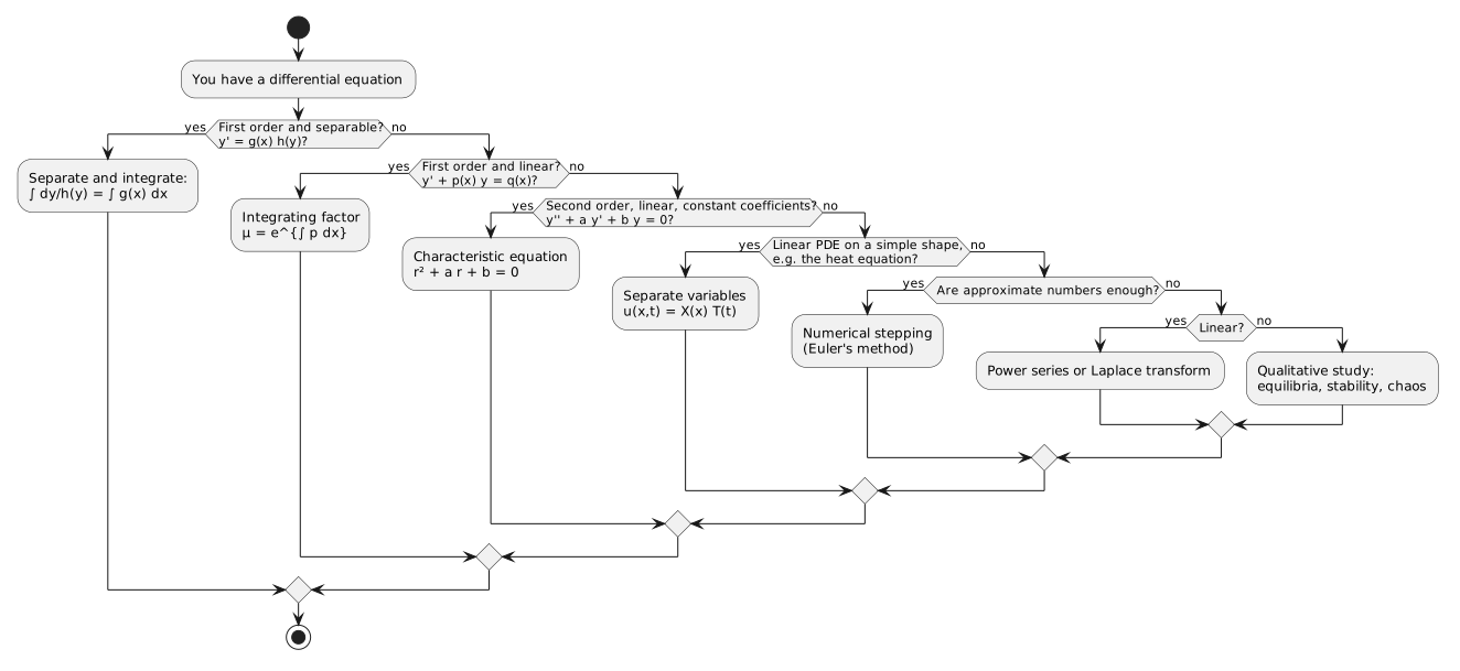
=== When no formula exists === | |||
Most equations, especially nonlinear ones, have no solution in terms of familiar functions. They are studied in one of three ways:<ref>{{#cite:Q1576}}</ref><ref>{{#cite:Q1578}}</ref> | |||
* '''Numerically''', when numbers suffice: [[Euler's method]] steps along the slope field; | |||
* '''[[Qualitative methods]]''': equilibria, stability and long-term behaviour, without formulas; | |||
* '''Series and transforms''', for linear cases: [[Power series]] or the [[Laplace transform]]. | |||
<uml type="uml"> | <uml type="uml"> | ||
| Line 355: | Line 242: | ||
start | start | ||
:You have a differential equation; | :You have a differential equation; | ||
if ( | if (First order and separable?\ny' = g(x) h(y)?) then (yes) | ||
:Separate and integrate:\n∫ dy/h(y) = ∫ g(x) dx; | :Separate and integrate:\n∫ dy/h(y) = ∫ g(x) dx; | ||
else (no) | else (no) | ||
if ( | if (First order and linear?\ny' + p(x) y = q(x)?) then (yes) | ||
: | :Integrating factor\nμ = e^{∫ p dx}; | ||
else (no) | else (no) | ||
if ( | if (Second order, linear, constant coefficients?\ny'' + a y' + b y = 0?) then (yes) | ||
: | :Characteristic equation\nr² + a r + b = 0; | ||
else (no) | else (no) | ||
if ( | if (Linear PDE on a simple shape,\ne.g. the heat equation?) then (yes) | ||
:Separate | :Separate variables\nu(x,t) = X(x) T(t); | ||
else (no) | else (no) | ||
if (Are approximate numbers enough?) then (yes) | if (Are approximate numbers enough?) then (yes) | ||
: | :Numerical stepping\n(Euler's method); | ||
else (no) | else (no) | ||
if ( | if (Linear?) then (yes) | ||
:Power series or Laplace transform | :Power series or Laplace transform; | ||
else (no) | else (no) | ||
: | :Qualitative study:\nequilibria, stability, chaos; | ||
endif | endif | ||
endif | endif | ||
| Line 383: | Line 270: | ||
@enduml | @enduml | ||
</uml> | </uml> | ||
== A short history == | == A short history == | ||
Differential equations | Differential equations came with the calculus. Newton's laws in the ''Principia'' (1687) are differential equations; Leibniz's notation $dy/dx$ (1670s) is the one still used. In the mid-18th century [[Person:Leonhard Euler|Leonhard Euler]] made the subject systematic, contributing the exponential trial solution, series methods, and the first numerical scheme, Euler's method.<ref>{{#cite:Q1577}}</ref> Physics supplied the PDEs: [[Person:Jean le Rond d'Alembert|Jean le Rond d'Alembert]] solved the vibrating-string (wave) equation in 1747, and [[Person:Joseph Fourier|Joseph Fourier]] derived and solved the heat equation in 1822 by expanding initial data in sine series, founding Fourier analysis.<ref>{{#cite:Q1579}}</ref> When no formula exists, behaviour can still be studied: [[Person:Henri Poincaré|Henri Poincaré]] pioneered this qualitative view on the three-body problem, and in 1963 [[Person:Edward Lorenz|Edward Lorenz]] found chaos in a three-equation model of convection, ending hopes of long-term weather prediction.<ref>{{#cite:Q1578}}</ref> | ||
[[File:Isaac Newton portrait.jpg|thumb|left|Isaac Newton (after Godfrey Kneller, 1689). Credit: James Thronill (public domain).]] | |||
[[File:Leonhard Euler portrait.jpg|thumb|Leonhard Euler (by Jakob Emanuel Handmann, 1753). Credit: Jakob Emanuel Handmann (public domain).]] | |||
== References == | == References == | ||
Revision as of 18:55, 5 September 2026
A differential equation is an equation whose unknown is a function and which also involves that function's derivatives (rates of change). Where an ordinary equation such as $x^2=9$ is solved by numbers, a differential equation such as $y'+2y=0$ is solved by functions $y(x)$. Laws of nature state how quantities change, so differential equations describe pendulums, cooling drinks, growing populations, and discharging capacitors. This article covers the standard exact solution methods, each with a worked numerical example, and the numerical, series, and qualitative routes used when no exact formula exists. It treats ordinary differential equations (one independent variable) and, briefly, partial differential equations (several).
A first example: slopes and a family of solutions
The simplest differential equation prescribes the slope of a function $y(x)$:
$$\frac{dy}{dx}=2x$$
Integration inverts differentiation, so integrating both sides gives
$$\int\frac{dy}{dx}\,dx=\int 2x\,dx\qquad\Longrightarrow\qquad y(x)=x^{2}+C$$
Every $C$ works, since $\frac{d}{dx}\left(x^2+C\right)=2x$; the solutions form the parabola family $y=x^2+C$, the general solution.
An extra condition picks out one member. If $y(0)=3$, then
$$3=0^2+C\qquad\Longrightarrow\qquad C=3\qquad\Longrightarrow\qquad y=x^2+3$$
Such a prescribed value is an initial condition.
Classifying differential equations
Three features decide how to solve an equation: its order, its linearity, and how many independent variables it involves.
Order
The order is the order of the highest derivative present. $dy/dx=2x$ is first order; Newton's second law,
is second order ($x(t)$ position of mass $m$, $F$ net force). An nth-order equation has $n$ arbitrary constants in its general solution, fixed by $n$ conditions, one constant appearing at each integration. Free fall shows the pattern: with only gravity $F_g=-mg$, Newton's law gives
$$m\frac{d^{2}x}{dt^{2}}=-mg\qquad\Longrightarrow\qquad\frac{d^{2}x}{dt^{2}}=-g\qquad(g\approx 9.8\ \mathrm{m\,s^{-2}})$$
Integrate once (constant $v_0$, the speed at $t=0$), then again (constant $x_0$, the height at $t=0$):
$$\frac{dx}{dt}=-gt+v_{0}\qquad\Longrightarrow\qquad x(t)=-\frac{g}{2}t^{2}+v_{0}t+x_{0}$$
Two initial conditions are needed. A ball dropped from rest at height $19.6\ \mathrm{m}$ hits the ground ($x=0$) when
$$0=19.6-4.9\,t^{2}\qquad\Longrightarrow\qquad t=\sqrt{19.6/4.9}=2\ \text{s}$$
Linearity and homogeneity
An equation is linear when the unknown and its derivatives appear only to the first power and never multiplied together. A linear first-order equation can always be written
$$\frac{dy}{dx}+p(x)\,y=q(x)$$
and is homogeneous when $q(x)=0$. The equations $dy/dx=y^2$ and $d^2\theta/dt^2+\sin\theta=0$ are nonlinear (square of $y$; sine of $\theta$).
If $y_1,y_2$ solve a homogeneous linear equation, so does $c_1y_1+c_2y_2$ (the superposition principle). Nonlinear equations lack this property. Superposition underlies every linear method below.
Ordinary and partial
An ordinary differential equation (ODE) has one independent variable. A partial differential equation (PDE) has several, with partial derivatives; for example the temperature $u(x,t)$ of an insulated metal bar obeys the heat equation
where $\alpha$ is the thermal diffusivity. The equation says a spot cools fastest where the temperature profile is most curved ($\partial^2u/\partial x^2$ large).
Slope fields
A first-order equation can be written
assigning to each point $(x,y)$ the slope $f(x,y)$ a solution must have there. Drawing short segments of that slope gives a direction field; solution curves run tangent to it.

Numerical methods such as Euler's method follow the field: read the slope, step a short distance along it, repeat.[1]
Solving differential equations
Separation of variables
A first-order equation is separable when the right-hand side factors into a function of $x$ times a function of $y$:
Divide by $h(y)$ and integrate; all $y$'s land on one side, all $x$'s on the other.
Exponential growth and decay
When a quantity changes at a rate proportional to its own size,
divide by $y$ and integrate:
$$\int\frac{dy}{y}=\int k\,dt\qquad\Longrightarrow\qquad \ln|y|=kt+C$$
Exponentiating, $|y|=e^C e^{kt}$; the sign of $y$ never changes, so absorbing it into the constant and writing $y(0)=y_0$,
With numbers: €1000 at 5% interest compounded continuously ($k=0.05\ \text{yr}^{-1}$) gives $y(t)=1000\,e^{0.05t}$, and
$$y(10)=1000\,e^{0.5}\approx 1648.7$$
Doubling time: $1000\,e^{0.05t}=2000\Rightarrow t=\ln 2/0.05\approx 13.9$ years. For $k<0$ the same solution describes decay; the half-life $y=y_0/2$ is $t_{1/2}=(\ln 2)/(-k)$.
Newton's law of cooling
A body hotter than its surroundings cools at a rate proportional to the temperature gap:
Separate and integrate:
$$\int\frac{dT}{T-T_a}=\int-k\,dt\qquad\Longrightarrow\qquad \ln|T-T_a|=-kt+C$$
Exponentiating and folding the (constant-sign) factor $T-T_a$ into the constant, with $T(0)=T_0$:
$$T(t)=T_a+(T_0-T_a)e^{-kt}$$
The gap $T-T_a$ decays exponentially, not $T$ itself. Example: a drink at $80\,^{\circ}\mathrm{C}$ in a $20\,^{\circ}\mathrm{C}$ room, $k=0.1\ \text{min}^{-1}$:
$$T(t)=20+60\,e^{-0.1t}$$
Reaches $40\,^{\circ}\mathrm{C}$ when $20+60e^{-0.1t}=40$, i.e. $t=10\ln 3\approx 11$ min.[1]
First-order linear equations: the integrating factor
For $y'+p(x)y=q(x)$ that is not separable, multiply by $\mu(x)$ chosen so the left side is a single derivative $(\mu y)'$. The product rule gives $(\mu y)'=\mu y'+\mu' y$, while multiplying the equation by $\mu$ gives $\mu y'+\mu p\,y$; matching coefficients requires $\mu'=p\mu$, whose solution is
$$\mu(x)=e^{\int p(x)\,dx}$$
Multiplying the equation by $\mu$,
so both sides integrate directly:
$$\mu(x)\,y=\int\mu(x)\,q(x)\,dx+C$$
Example: $y'+y=e^{-x}$. Here $p=1$, $\mu=e^x$, and
$$e^x y'+e^x y=1\qquad\Longrightarrow\qquad (e^x y)'=1\qquad\Longrightarrow\qquad e^x y=x+C\qquad\Longrightarrow\qquad y=(x+C)e^{-x}$$
The condition $y(0)=2$ gives $C=2$.[1][2]
Constant-coefficient linear equations of order two
The equation $y''+a\,y'+b\,y=0$ (constant coefficients) models a mass on a spring, a small-angle pendulum, and an RLC circuit. It is solved by trying an exponential $y=e^{rx}$, since $y'=re^{rx}$ and $y''=r^2e^{rx}$:
Substitution turns the equation into algebra: $(r^2+ar+b)e^{rx}=0$, and $e^{rx}\neq 0$, so
$$r^2+ar+b=0$$
This is the characteristic equation; its roots determine the solution:
- distinct real roots $r_1\neq r_2$: $y=C_1e^{r_1x}+C_2e^{r_2x}$;
- one repeated root $r$: $y=(C_1+C_2x)e^{rx}$;
- complex pair $r=\alpha\pm i\beta$: $y=e^{\alpha x}(C_1\cos\beta x+C_2\sin\beta x)$.
Example ($y''-3y'+2y=0$): $r^2-3r+2=(r-1)(r-2)$, so
Each term checks: for $y=e^x$, $y''-3y'+2y=(1-3+2)e^x=0$.
The harmonic oscillator (a mass on a spring)
A mass displaced $x$ from rest is pulled back by $-kx$ (Hooke's law), so Newton's second law gives
$$m\frac{d^2x}{dt^2}=-kx\qquad\Longrightarrow\qquad x''+\frac{k}{m}x=0$$
With $\omega_0^2=k/m$ this is the harmonic oscillator equation
Its characteristic equation $r^2+\omega_0^2=0$ has roots $\pm i\omega_0$, the complex case above ($\alpha=0$). Since $\frac{d^2}{dt^2}\cos\omega_0 t=-\omega_0^2\cos\omega_0 t$, and likewise for sine, superposition gives
$$x(t)=A\cos\omega_0 t+B\sin\omega_0 t$$
with $A,B$ fixed by the initial position and velocity.

Example: $m=2\ \mathrm{kg}$, $k=8\ \mathrm{N/m}$, so $\omega_0=\sqrt{8/2}=2\ \text{rad/s}$. Pulled $10\ \mathrm{cm}$ out and released from rest, $B=0$ and $x(t)=0.10\cos 2t$ metres. The period is
$$P=\frac{2\pi}{\omega_0}=\pi\approx 3.14\ \text{s}$$
and after one second
$$x(1)=0.10\cos 2\approx 0.10(-0.416)\approx -0.042\ \text{m}$$
Such fixed-amplitude sinusoidal motion is simple harmonic motion.[2]
Partial differential equations: separating variables in the heat equation
Solve the heat equation on a bar of length $L$, insulated sides, ends held at $0$:
$$\frac{\partial u}{\partial t}=\alpha\frac{\partial^2u}{\partial x^2}$$
Seek a product solution $u(x,t)=X(x)T(t)$. Substitution gives $XT'=\alpha X''T$; dividing by $\alpha XT$,
The left side depends only on $t$, the right only on $x$, so both equal one constant, $-\lambda$. This yields two ODEs,
$$T'=-\alpha\lambda T\qquad\Longrightarrow\qquad T=e^{-\alpha\lambda t}$$
$$X''=-\lambda X\qquad\Longrightarrow\qquad X=A\cos(\sqrt{\lambda}\,x)+B\sin(\sqrt{\lambda}\,x)$$
The end conditions $u(0,t)=u(L,t)=0$ force $X(0)=X(L)=0$: hence $A=0$ and $\sin(\sqrt\lambda\,L)=0$, so $\sqrt\lambda\,L=n\pi$, $n=1,2,\dots$ Each allowed $\lambda=(n\pi/L)^2$ gives one mode
$$u_n(x,t)=\sin\frac{n\pi x}{L}\,e^{-\alpha(n\pi/L)^2t}$$
The equation is linear and homogeneous, so superposition applies, and the general solution is
with the $b_n$ fixed by the initial profile $u(x,0)$ (a Fourier sine series). Modes with many wiggles (large $n$) decay fastest, since the decay rate $\alpha(n\pi/L)^2$ grows like $n^2$; soon only the $n=1$ mode remains.
Numbers: a $1\ \mathrm{m}$ iron bar, $\alpha\approx 2.3\times10^{-5}\ \mathrm{m^2s^{-1}}$, heated so $u(x,0)=100\sin(\pi x/L)$ (ends at $0\,^{\circ}\mathrm{C}$, centre $100\,^{\circ}\mathrm{C}$). Only $n=1$ is present:
$$u(x,t)=100\sin\frac{\pi x}{L}\,e^{-\alpha\pi^2t/L^2}$$
At the centre, with $L=1$ and $\alpha\pi^2\approx 2.3\times10^{-4}\ \text{s}^{-1}$,
$$u\!\left(\tfrac12,t\right)=100\,e^{-2.3\times10^{-4}t}$$
so after one hour $u\approx 100e^{-0.82}\approx 44\,^{\circ}\mathrm{C}$, and $50\,^{\circ}\mathrm{C}$ is reached at $t=\ln 2/(2.3\times10^{-4})\approx 3050\ \text{s}\approx 51$ min.[3]
When no formula exists
Most equations, especially nonlinear ones, have no solution in terms of familiar functions. They are studied in one of three ways:[1][4]
- Numerically, when numbers suffice: Euler's method steps along the slope field;
- Qualitative methods: equilibria, stability and long-term behaviour, without formulas;
- Series and transforms, for linear cases: Power series or the Laplace transform.
A short history
Differential equations came with the calculus. Newton's laws in the Principia (1687) are differential equations; Leibniz's notation $dy/dx$ (1670s) is the one still used. In the mid-18th century Leonhard Euler made the subject systematic, contributing the exponential trial solution, series methods, and the first numerical scheme, Euler's method.[2] Physics supplied the PDEs: Jean le Rond d'Alembert solved the vibrating-string (wave) equation in 1747, and Joseph Fourier derived and solved the heat equation in 1822 by expanding initial data in sine series, founding Fourier analysis.[3] When no formula exists, behaviour can still be studied: Henri Poincaré pioneered this qualitative view on the three-body problem, and in 1963 Edward Lorenz found chaos in a three-equation model of convection, ending hopes of long-term weather prediction.[4]


References
- ↑ ↑ ↑ ↑ Boyce, W. E. (2012). Elementary Differential Equations and Boundary Value Problems (Book). In Elementary Differential Equations and Boundary Value Problems (Book). John Wiley & Sons.
- ↑ ↑ ↑ Tenenbaum, M. (1985). Ordinary Differential Equations (Book). In Ordinary Differential Equations (Book). Dover Publications.
- ↑ ↑ Strauss, W. A. (2008). Partial Differential Equations: An Introduction (Book). In Partial Differential Equations: An Introduction (Book). John Wiley & Sons.
- ↑ ↑ Strogatz, S. H. (2015). Nonlinear Dynamics and Chaos: With Applications to Physics, Biology, Chemistry, and Engineering (Book). In Nonlinear Dynamics and Chaos: With Applications to Physics, Biology, Chemistry, and Engineering (Book). Westview Press.
Further reading
- Differential equation, Wikipedia
- Differential Equation, Wolfram MathWorld
- 18.03SC Differential Equations, MIT OpenCourseWare
- Leonhard Euler, MacTutor History of Mathematics