Differential equation
A differential equation is an equation whose unknown is a function and which also involves that function's derivatives (rates of change). Where an ordinary equation such as $x^2=9$ is solved by numbers, a differential equation such as $y'+2y=0$ is solved by functions $y(x)$. Laws of nature state how quantities change, so differential equations describe pendulums, cooling drinks, growing populations, and discharging capacitors. This article covers the standard exact solution methods, each with a worked numerical example, and the numerical, series, and qualitative routes used when no exact formula exists. It treats ordinary differential equations (one independent variable) and, briefly, partial differential equations (several).
A first example: slopes and a family of solutions
The simplest differential equation prescribes the slope of a function $y(x)$:
$$\frac{dy}{dx}=2x$$
Integration inverts differentiation, so integrating both sides gives
$$\int\frac{dy}{dx}\,dx=\int 2x\,dx\qquad\Longrightarrow\qquad y(x)=x^{2}+C$$
Every $C$ works, since $\frac{d}{dx}\left(x^2+C\right)=2x$; the solutions form the parabola family $y=x^2+C$, the general solution.
An extra condition picks out one member. If $y(0)=3$, then
$$3=0^2+C\qquad\Longrightarrow\qquad C=3\qquad\Longrightarrow\qquad y=x^2+3$$
Such a prescribed value is an initial condition.
Classifying differential equations
Three features decide how to solve an equation: its order, its linearity, and how many independent variables it involves.
Order
The order is the order of the highest derivative present. $dy/dx=2x$ is first order; Newton's second law,
is second order ($x(t)$ position of mass $m$, $F$ net force). An nth-order equation has $n$ arbitrary constants in its general solution, fixed by $n$ conditions, one constant appearing at each integration. Free fall shows the pattern: with only gravity $F_g=-mg$, Newton's law gives
$$m\frac{d^{2}x}{dt^{2}}=-mg\qquad\Longrightarrow\qquad\frac{d^{2}x}{dt^{2}}=-g\qquad(g\approx 9.8\ \mathrm{m\,s^{-2}})$$
Integrate once (constant $v_0$, the speed at $t=0$), then again (constant $x_0$, the height at $t=0$):
$$\frac{dx}{dt}=-gt+v_{0}\qquad\Longrightarrow\qquad x(t)=-\frac{g}{2}t^{2}+v_{0}t+x_{0}$$
Two initial conditions are needed. A ball dropped from rest at height $19.6\ \mathrm{m}$ hits the ground ($x=0$) when
$$0=19.6-4.9\,t^{2}\qquad\Longrightarrow\qquad t=\sqrt{19.6/4.9}=2\ \text{s}$$
Linearity and homogeneity
An equation is linear when the unknown and its derivatives appear only to the first power and never multiplied together. A linear first-order equation can always be written
$$\frac{dy}{dx}+p(x)\,y=q(x)$$
and is homogeneous when $q(x)=0$. The equations $dy/dx=y^2$ and $d^2\theta/dt^2+\sin\theta=0$ are nonlinear (square of $y$; sine of $\theta$).
If $y_1,y_2$ solve a homogeneous linear equation, so does $c_1y_1+c_2y_2$ (the superposition principle). Nonlinear equations lack this property. Superposition underlies every linear method below.
Ordinary and partial
An ordinary differential equation (ODE) has one independent variable. A partial differential equation (PDE) has several, with partial derivatives; for example the temperature $u(x,t)$ of an insulated metal bar obeys the heat equation
where $\alpha$ is the thermal diffusivity. The equation says a spot cools fastest where the temperature profile is most curved ($\partial^2u/\partial x^2$ large).
Slope fields
A first-order equation can be written
assigning to each point $(x,y)$ the slope $f(x,y)$ a solution must have there. Drawing short segments of that slope gives a direction field; solution curves run tangent to it.

Numerical methods such as Euler's method follow the field: read the slope, step a short distance along it, repeat.[1]
Solving differential equations
Separation of variables
A first-order equation is separable when the right-hand side factors into a function of $x$ times a function of $y$:
Divide by $h(y)$ and integrate; all $y$'s land on one side, all $x$'s on the other.
Exponential growth and decay
When a quantity changes at a rate proportional to its own size,
divide by $y$ and integrate:
$$\int\frac{dy}{y}=\int k\,dt\qquad\Longrightarrow\qquad \ln|y|=kt+C$$
Exponentiating, $|y|=e^C e^{kt}$; the sign of $y$ never changes, so absorbing it into the constant and writing $y(0)=y_0$,
With numbers: €1000 at 5% interest compounded continuously ($k=0.05\ \text{yr}^{-1}$) gives $y(t)=1000\,e^{0.05t}$, and
$$y(10)=1000\,e^{0.5}\approx 1648.7$$
Doubling time: $1000\,e^{0.05t}=2000\Rightarrow t=\ln 2/0.05\approx 13.9$ years. For $k<0$ the same solution describes decay; the half-life $y=y_0/2$ is $t_{1/2}=(\ln 2)/(-k)$.
Newton's law of cooling
A body hotter than its surroundings cools at a rate proportional to the temperature gap:
Separate and integrate:
$$\int\frac{dT}{T-T_a}=\int-k\,dt\qquad\Longrightarrow\qquad \ln|T-T_a|=-kt+C$$
Exponentiating and folding the (constant-sign) factor $T-T_a$ into the constant, with $T(0)=T_0$:
$$T(t)=T_a+(T_0-T_a)e^{-kt}$$
The gap $T-T_a$ decays exponentially, not $T$ itself. Example: a drink at $80\,^{\circ}\mathrm{C}$ in a $20\,^{\circ}\mathrm{C}$ room, $k=0.1\ \text{min}^{-1}$:
$$T(t)=20+60\,e^{-0.1t}$$
Reaches $40\,^{\circ}\mathrm{C}$ when $20+60e^{-0.1t}=40$, i.e. $t=10\ln 3\approx 11$ min.[1]
First-order linear equations: the integrating factor
For $y'+p(x)y=q(x)$ that is not separable, multiply by $\mu(x)$ chosen so the left side is a single derivative $(\mu y)'$. The product rule gives $(\mu y)'=\mu y'+\mu' y$, while multiplying the equation by $\mu$ gives $\mu y'+\mu p\,y$; matching coefficients requires $\mu'=p\mu$, whose solution is
$$\mu(x)=e^{\int p(x)\,dx}$$
Multiplying the equation by $\mu$,
so both sides integrate directly:
$$\mu(x)\,y=\int\mu(x)\,q(x)\,dx+C$$
Example: $y'+y=e^{-x}$. Here $p=1$, $\mu=e^x$, and
$$e^x y'+e^x y=1\qquad\Longrightarrow\qquad (e^x y)'=1\qquad\Longrightarrow\qquad e^x y=x+C\qquad\Longrightarrow\qquad y=(x+C)e^{-x}$$
The condition $y(0)=2$ gives $C=2$.[1][2]
Constant-coefficient linear equations of order two
The equation $y''+a\,y'+b\,y=0$ (constant coefficients) models a mass on a spring, a small-angle pendulum, and an RLC circuit. It is solved by trying an exponential $y=e^{rx}$, since $y'=re^{rx}$ and $y''=r^2e^{rx}$:
Substitution turns the equation into algebra: $(r^2+ar+b)e^{rx}=0$, and $e^{rx}\neq 0$, so
$$r^2+ar+b=0$$
This is the characteristic equation; its roots determine the solution:
- distinct real roots $r_1\neq r_2$: $y=C_1e^{r_1x}+C_2e^{r_2x}$;
- one repeated root $r$: $y=(C_1+C_2x)e^{rx}$;
- complex pair $r=\alpha\pm i\beta$: $y=e^{\alpha x}(C_1\cos\beta x+C_2\sin\beta x)$.
Example ($y''-3y'+2y=0$): $r^2-3r+2=(r-1)(r-2)$, so
Each term checks: for $y=e^x$, $y''-3y'+2y=(1-3+2)e^x=0$.
The harmonic oscillator (a mass on a spring)
A mass displaced $x$ from rest is pulled back by $-kx$ (Hooke's law), so Newton's second law gives
$$m\frac{d^2x}{dt^2}=-kx\qquad\Longrightarrow\qquad x''+\frac{k}{m}x=0$$
With $\omega_0^2=k/m$ this is the harmonic oscillator equation
Its characteristic equation $r^2+\omega_0^2=0$ has roots $\pm i\omega_0$, the complex case above ($\alpha=0$). Since $\frac{d^2}{dt^2}\cos\omega_0 t=-\omega_0^2\cos\omega_0 t$, and likewise for sine, superposition gives
$$x(t)=A\cos\omega_0 t+B\sin\omega_0 t$$
with $A,B$ fixed by the initial position and velocity.

Example: $m=2\ \mathrm{kg}$, $k=8\ \mathrm{N/m}$, so $\omega_0=\sqrt{8/2}=2\ \text{rad/s}$. Pulled $10\ \mathrm{cm}$ out and released from rest, $B=0$ and $x(t)=0.10\cos 2t$ metres. The period is
$$P=\frac{2\pi}{\omega_0}=\pi\approx 3.14\ \text{s}$$
and after one second
$$x(1)=0.10\cos 2\approx 0.10(-0.416)\approx -0.042\ \text{m}$$
Such fixed-amplitude sinusoidal motion is simple harmonic motion.[2]
Partial differential equations: separating variables in the heat equation
Solve the heat equation on a bar of length $L$, insulated sides, ends held at $0$:
$$\frac{\partial u}{\partial t}=\alpha\frac{\partial^2u}{\partial x^2}$$
Seek a product solution $u(x,t)=X(x)T(t)$. Substitution gives $XT'=\alpha X''T$; dividing by $\alpha XT$,
The left side depends only on $t$, the right only on $x$, so both equal one constant, $-\lambda$. This yields two ODEs,
$$T'=-\alpha\lambda T\qquad\Longrightarrow\qquad T=e^{-\alpha\lambda t}$$
$$X''=-\lambda X\qquad\Longrightarrow\qquad X=A\cos(\sqrt{\lambda}\,x)+B\sin(\sqrt{\lambda}\,x)$$
The end conditions $u(0,t)=u(L,t)=0$ force $X(0)=X(L)=0$: hence $A=0$ and $\sin(\sqrt\lambda\,L)=0$, so $\sqrt\lambda\,L=n\pi$, $n=1,2,\dots$ Each allowed $\lambda=(n\pi/L)^2$ gives one mode
$$u_n(x,t)=\sin\frac{n\pi x}{L}\,e^{-\alpha(n\pi/L)^2t}$$
The equation is linear and homogeneous, so superposition applies, and the general solution is
with the $b_n$ fixed by the initial profile $u(x,0)$ (a Fourier sine series). Modes with many wiggles (large $n$) decay fastest, since the decay rate $\alpha(n\pi/L)^2$ grows like $n^2$; soon only the $n=1$ mode remains.
Numbers: a $1\ \mathrm{m}$ iron bar, $\alpha\approx 2.3\times10^{-5}\ \mathrm{m^2s^{-1}}$, heated so $u(x,0)=100\sin(\pi x/L)$ (ends at $0\,^{\circ}\mathrm{C}$, centre $100\,^{\circ}\mathrm{C}$). Only $n=1$ is present:
$$u(x,t)=100\sin\frac{\pi x}{L}\,e^{-\alpha\pi^2t/L^2}$$
At the centre, with $L=1$ and $\alpha\pi^2\approx 2.3\times10^{-4}\ \text{s}^{-1}$,
$$u\!\left(\tfrac12,t\right)=100\,e^{-2.3\times10^{-4}t}$$
so after one hour $u\approx 100e^{-0.82}\approx 44\,^{\circ}\mathrm{C}$, and $50\,^{\circ}\mathrm{C}$ is reached at $t=\ln 2/(2.3\times10^{-4})\approx 3050\ \text{s}\approx 51$ min.[3]
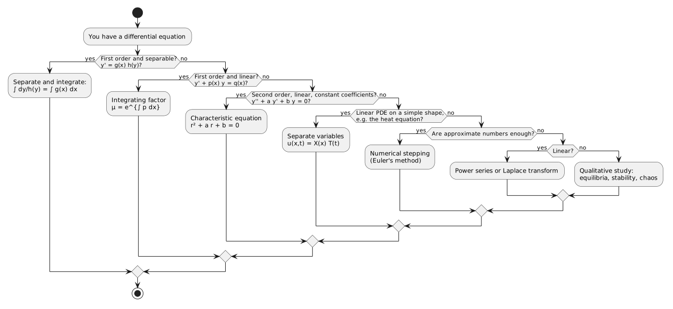
When no formula exists
Most equations, especially nonlinear ones, have no solution in terms of familiar functions. They are studied in one of three ways:[1][4]
- Numerically, when numbers suffice: Euler's method steps along the slope field;
- Qualitative methods: equilibria, stability and long-term behaviour, without formulas;
- Series and transforms, for linear cases: Power series or the Laplace transform.
A short history
Differential equations came with the calculus. Newton's laws in the Principia (1687) are differential equations; Leibniz's notation $dy/dx$ (1670s) is the one still used. In the mid-18th century Leonhard Euler made the subject systematic, contributing the exponential trial solution, series methods, and the first numerical scheme, Euler's method.[2] Physics supplied the PDEs: Jean le Rond d'Alembert solved the vibrating-string (wave) equation in 1747, and Joseph Fourier derived and solved the heat equation in 1822 by expanding initial data in sine series, founding Fourier analysis.[3] When no formula exists, behaviour can still be studied: Henri Poincaré pioneered this qualitative view on the three-body problem, and in 1963 Edward Lorenz found chaos in a three-equation model of convection, ending hopes of long-term weather prediction.[4]


References
- ↑ ↑ ↑ ↑ Boyce, W. E. (2012). Elementary Differential Equations and Boundary Value Problems (Book). In Elementary Differential Equations and Boundary Value Problems (Book). John Wiley & Sons.
- ↑ ↑ ↑ Tenenbaum, M. (1985). Ordinary Differential Equations (Book). In Ordinary Differential Equations (Book). Dover Publications.
- ↑ ↑ Strauss, W. A. (2008). Partial Differential Equations: An Introduction (Book). In Partial Differential Equations: An Introduction (Book). John Wiley & Sons.
- ↑ ↑ Strogatz, S. H. (2015). Nonlinear Dynamics and Chaos: With Applications to Physics, Biology, Chemistry, and Engineering (Book). In Nonlinear Dynamics and Chaos: With Applications to Physics, Biology, Chemistry, and Engineering (Book). Westview Press.
Further reading
- Differential equation, Wikipedia
- Differential Equation, Wolfram MathWorld
- 18.03SC Differential Equations, MIT OpenCourseWare
- Leonhard Euler, MacTutor History of Mathematics