Differential equation

Languages: English · français · Esperanto

A differential equation is an equation that relates an unknown function to its own derivatives. An algebraic equation such as x² − 3x + 2 = 0 asks for numbers; a differential equation asks for functions. Because a derivative measures how fast a quantity changes, differential equations describe change itself, and they form the mathematical language of much of science and engineering: the fall of a body, the swing of a pendulum, the decay of a radioactive nucleus, the flow of heat in a rod, the vibration of a string and the growth of a population are all described by differential equations.^[1]^[2]

A few features are common to all differential equations:

the unknown is a function, not a number;
a solution is rarely unique: it is a family of functions containing arbitrary constants, and a particular member is singled out by extra conditions, such as the state of the system at some starting time;
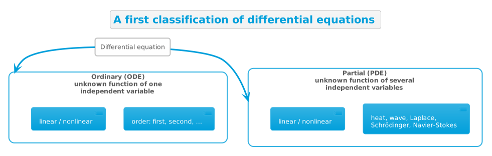
they are classified as ordinary or partial, by their order, and as linear or nonlinear.

Types of differential equations

Ordinary and partial differential equations

If the unknown function depends on a single independent variable, only ordinary derivatives occur, and the equation is an ordinary differential equation (ODE). Writing the unknown as y(x), an ODE can be expressed in implicit form as a relation between the independent variable, the function, and its derivatives up to some order n:

F\bigl(x,y,y',y'',\ldots,y^{(n)}\bigr)=0

where F is a given function. If the equation can be solved for the highest derivative, it takes an explicit form, for a first-order equation:

\frac{dy}{dx}=f(x,y)

The right-hand side f(x, y) prescribes, at every point (x, y), the slope that the graph of a solution must have as it passes through that point.

If the unknown function depends on two or more variables and partial derivatives appear, the equation is a partial differential equation (PDE). PDEs govern fields, quantities that vary from point to point and, often, with time. The classical linear examples are the heat equation, the wave equation and Laplace's equation:

\frac{\partial u}{\partial t}=\alpha\frac{\partial^{2}u}{\partial x^{2}}

\frac{\partial^{2}u}{\partial t^{2}}=c^{2}\frac{\partial^{2}u}{\partial x^{2}}

\frac{\partial^{2}u}{\partial x^{2}}+\frac{\partial^{2}u}{\partial y^{2}}=0

In the wave equation u(x, t) is the displacement of the string at position x and time t, and c is the wave speed; in the heat equation u is the temperature and α the thermal diffusivity; in Laplace's equation u is a potential in equilibrium, for instance a steady temperature or an electrostatic potential.^[2]

Order and linearity

The order of a differential equation is the order of the highest derivative that appears in it: an equation containing y⁽ⁿ⁾ but no higher derivative has order n. Newton's second law of motion is a second-order equation because it involves a second derivative, whereas the heat and wave equations are first order in time and second order in space.

A differential equation is linear if the unknown function and its derivatives occur only to the first power and are never multiplied together; otherwise it is nonlinear. Linear homogeneous equations obey the superposition principle: any linear combination of solutions is again a solution. This principle underlies the method of Fourier series for the heat and wave equations. Nonlinearity, by contrast, typically makes closed-form solution impossible and produces qualitatively new behaviour, as the model equations below illustrate.

Differential equations as mathematical models

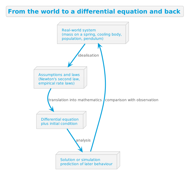
When a question from physics, biology, chemistry or economics is turned into mathematics, the quantities whose evolution matters become the unknown functions, and the laws connecting their rates of change to the quantities themselves become differential equations. Together with a statement of the initial state, the resulting equation predicts the behaviour of the system at all later times.^[1]^[3]

Mechanics

Newton's second law of motion states that the acceleration of a body is proportional to the net force acting on it:

m\frac{d^{2}x}{dt^{2}}=F

where x(t) is the position of the body, m its mass, and the force F may itself depend on time, position and velocity. For a mass attached to a spring whose restoring force is linear in the displacement, this becomes the harmonic oscillator equation:

\frac{d^{2}x}{dt^{2}}+\omega_{0}^{2}x=0

whose solutions are sinusoidal oscillations at the natural frequency ω₀; such motion is called simple harmonic motion.

Growth, decay and heat transfer

A quantity that changes at a rate proportional to its current size satisfies the exponential growth and decay equation:

\frac{dy}{dt}=k\,y

Its solutions are exponentials:

y(t)=y_{0}\,e^{kt}

so a population with unlimited resources grows exponentially (k > 0), whereas a radioactive substance, for which k < 0, decays exponentially towards zero. Newton's law of cooling describes a body whose temperature T differs from a constant ambient temperature Tₐ:

\frac{dT}{dt}=-k\bigl(T-T_{a}\bigr)

The temperature difference decays exponentially, so the body approaches the ambient temperature but never quite reaches it.^[1]

Real populations are not unlimited. The logistic equation adds a term that slows growth as the population P approaches a carrying capacity K:

\frac{dP}{dt}=rP\Bigl(1-\frac{P}{K}\Bigr)

where r is the intrinsic growth rate. Solutions rise from a small initial population and level off at K, giving the characteristic S-shaped curve of logistic growth.^[1]

A nonlinear example: the pendulum

An ideal pendulum, a mass on a rigid rod of length L swinging under gravity, obeys

\frac{d^{2}\theta}{dt^{2}}+\frac{g}{L}\sin\theta=0

where θ is the angle from the vertical and g the gravitational acceleration. The equation is nonlinear because sin θ is not a linear function of θ. For small oscillations, sin θ ≈ θ, and the equation reduces to the harmonic oscillator equation with frequency √(g/L). For larger swings the nonlinearity matters: the period lengthens and, if damping or driving is added, the pendulum exhibits the whole range of nonlinear phenomena, from limit cycles to chaos.^[3]

Geometry of first-order equations

Direction fields

A first-order equation of the form dy/dx = f(x, y), as introduced above, assigns to every point (x, y) the slope that a solution curve must have there. Drawing a short line segment of that slope at many points produces a direction field (or slope field), and every solution curve is a curve that stays tangent to the segments everywhere. Direction fields make the qualitative behaviour of solutions visible even when no closed-form solution exists.^[1]

The illustration shows the direction field of the exponential equation dy/dx = y. The field makes visible both the growth of the solution curves and the fact that through every point, apart from the special constant solution y = 0, exactly one solution curve passes.

Existence and uniqueness

Because most differential equations cannot be solved in closed form, the first question about an equation is usually whether a solution exists and whether it is unique. This is asked for an initial value problem, which fixes the state of the system at a starting point x₀:

\frac{dy}{dx}=f(x,y),\qquad y(x_{0})=y_{0}

According to the Picard–Lindelöf theorem, if f is continuous in a neighbourhood of (x₀, y₀) and satisfies a Lipschitz condition in y there, then a unique solution exists on some interval containing x₀.^[1]^[4] If f is merely continuous, a solution is still guaranteed to exist (the Peano existence theorem), but uniqueness may fail: the problem dy/dx = 3y^⅔ with y(0) = 0 has two different solutions through the origin, namely y(x) = 0 and y(x) = x³, because the right-hand side is not Lipschitz continuous at y = 0.^[1]

Any explicit equation of order n can be rewritten as a system of n first-order equations by declaring the derivatives to be new unknown functions. This reduction to a first-order system is the starting point of most theory and of almost all numerical methods.^[1]

Solving differential equations

Analytical methods

For the relatively small class of equations that can be solved in closed form, a toolkit of classical methods exists:

first-order equations: separation of variables, integrating factors for linear equations, substitutions such as the Bernoulli substitution;
linear equations with constant coefficients: exponential trial solutions and the characteristic equation, variation of parameters;
equations with variable coefficients: power-series solutions about ordinary points and Frobenius series about regular singular points;
integral transforms, in particular the Laplace transform, which turns differential equations into algebraic ones;
for partial differential equations: separation of variables combined with Fourier series, and transform methods.

The theory of these methods is treated in standard textbooks on ordinary and partial differential equations.^[4]^[2] Still, only a minority of differential equations, almost all of them linear, can be solved explicitly; most equations that arise in applications are treated by numerical or qualitative methods.^[3]

Numerical methods

When no closed-form solution is available, solutions are approximated by numerical integration. The simplest scheme, Euler's method, advances an approximate solution yₙ at points xₙ = x₀ + nh by repeatedly applying one step:

y_{n+1}=y_{n}+h\,f(x_{n},y_{n})

More accurate and more stable methods, such as the Runge–Kutta family, are built on the same idea of using the differential equation to extrapolate from known values, and are implemented in essentially every numerical computing environment.^[1]

Qualitative methods

For nonlinear equations, and especially for systems of two or more equations, the geometry of solutions matters as much as their formulas. Qualitative analysis studies the equilibrium points at which the system does not change, the stability of those equilibria, and the way solutions flow between them in the phase plane; as parameters change, the behaviour can reorganise itself in bifurcations, and in three or more dimensions a system can settle onto a chaotic attractor, whose solutions are deterministic yet aperiodic and extremely sensitive to initial conditions.^[3]

History

Differential equations arose with the calculus that Isaac Newton and Gottfried Wilhelm Leibniz developed independently in the late 17th century. Newton's laws of motion and of universal gravitation, published in his Principia of 1687, are differential equations, and solving them explained the orbits of the planets; Leibniz introduced the notation dy/dx still used today. The first differential equations were solved by the brothers Jacob and Johann Bernoulli, and in the 18th century Leonhard Euler turned a collection of ad hoc tricks into a systematic theory, developing the general treatment of linear equations with constant coefficients, series methods, and the first numerical integration scheme, which still bears his name.^[4]^[1]

Alongside the theory of ordinary equations, the 18th and 19th centuries created the partial differential equations of physics. Jean le Rond d'Alembert wrote down and solved the one-dimensional wave equation for the vibrating string in the 1740s, and Joseph Fourier derived the heat equation from the physics of conduction and solved it with trigonometric series in his Théorie analytique de la chaleur of 1822, founding Fourier analysis.^[2]

Augustin-Louis Cauchy and, later, Rudolf Lipschitz and Émile Picard placed the existence and uniqueness of solutions on a rigorous footing in the 19th century.^[1] In the 20th century, Henri Poincaré's qualitative approach grew into the modern theory of dynamical systems: in 1963 the meteorologist Edward Lorenz found chaotic behaviour in a simple system of three differential equations modelling atmospheric convection, a landmark in the study of nonlinear dynamics.^[3] Since the middle of the 20th century, numerical computing has made differential equations the everyday working tool of science and engineering that they are today.

References

↑ ↑ ↑ ↑ ↑ ↑ ↑ ↑ ↑ ↑ ↑ Boyce, W. E. (2012). Elementary Differential Equations and Boundary Value Problems (Book). In Elementary Differential Equations and Boundary Value Problems (Book). John Wiley & Sons.
↑ ↑ ↑ ↑ Strauss, W. A. (2008). Partial Differential Equations: An Introduction (Book). In Partial Differential Equations: An Introduction (Book). John Wiley & Sons.
↑ ↑ ↑ ↑ ↑ Strogatz, S. H. (2015). Nonlinear Dynamics and Chaos: With Applications to Physics, Biology, Chemistry, and Engineering (Book). In Nonlinear Dynamics and Chaos: With Applications to Physics, Biology, Chemistry, and Engineering (Book). Westview Press.
↑ ↑ ↑ Tenenbaum, M. (1985). Ordinary Differential Equations (Book). In Ordinary Differential Equations (Book). Dover Publications.

Differential equation

Contents

Types of differential equations